Hilbert Spaces and Linear Operators

In this lesson we define Hilbert spaces precisely, first showing how and where they fit within the main branches of mathematics, namely algebra and topology. We will arrive at the classification theorem for Hilbert spaces: two Hilbert spaces are isometrically isomorphic if and only if they share the same Hilbertian dimension, a notion not to be confused with the algebraic dimension of a vector space, since these two only coincide in finite dimension. We will give the model reference spaces for each case (finite dimension, countably infinite dimension, and uncountably infinite dimension), with an overview of their use in elementary quantum mechanics. We will close with a discussion on whether or not the physics defined by Hilbert spaces related by isomorphisms is invariant.

1. Mathematical structures in physics

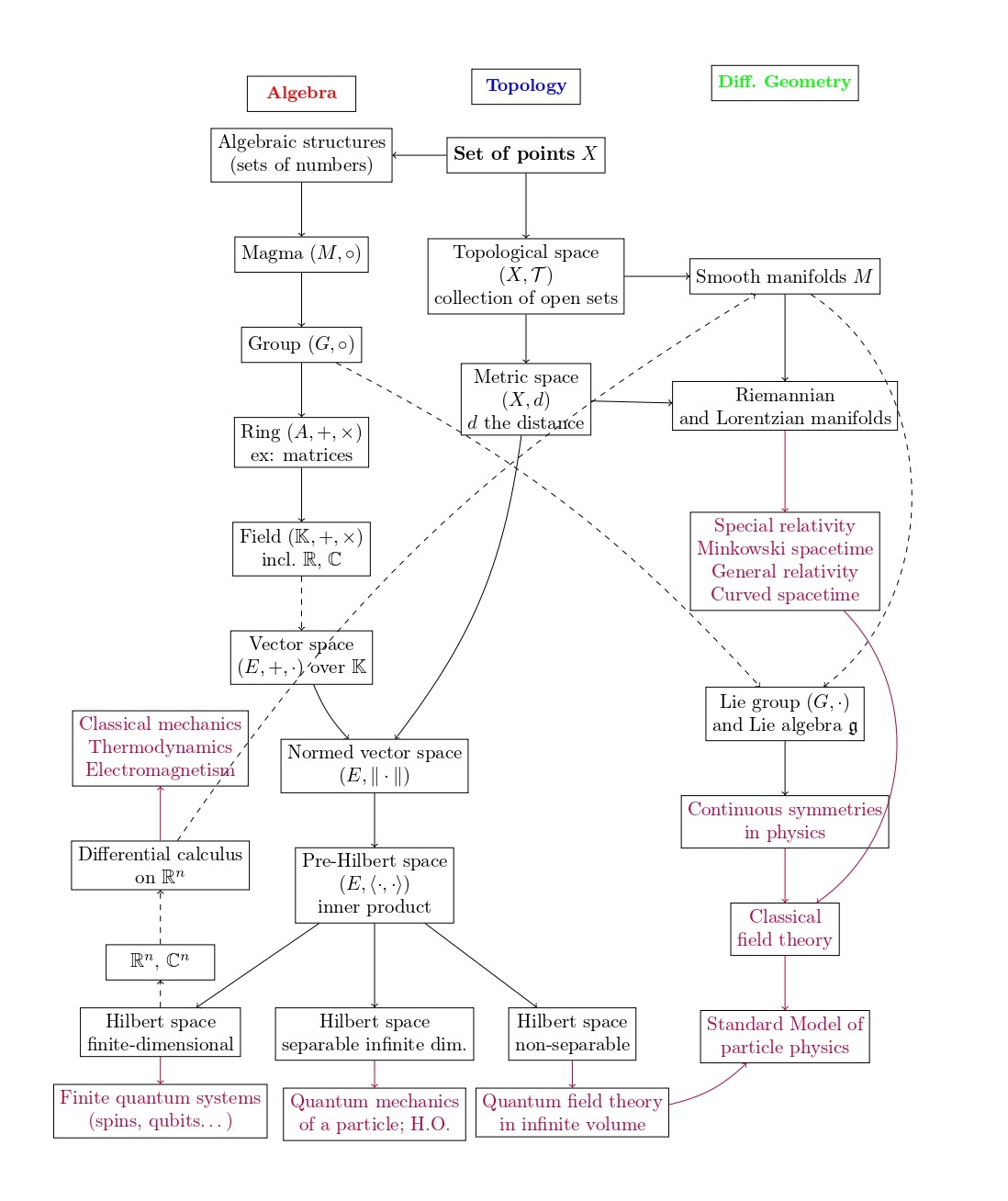
In order to reach Hilbert spaces ^[1,2], we give a brief review of the "map of mathematics" most commonly used in theoretical physics. The following page shows a highly simplified and largely incomplete version of such a map, but one that is sufficient for this course, cf. Figure (1).

If we start from the intuitive notion of a set of points¹, we proceed by gradually adding structure to this set. We will progressively explain this scheme in what follows.

1.1. Algebraic structures and vector spaces

Starting from sets of points, we can go directly into the left-hand branch of our map (1), that of algebraic structures, generally used to describe sets of numbers (but not only).

To do this, we add one or more internal composition laws to the set of points; as these laws satisfy certain rules (associativity, commutativity, existence of an identity element, etc.), we obtain specific structures.

In this figure, we represent some fundamental structures: the magma (a set equipped with an internal composition law without any particular property), groups, rings, and fields. Many others exist, such as semigroups, monoids, or non-commutative rings — but they are not shown here to keep the figure readable. Each of these structures specializes the previous one: every field is a ring, every ring is a group for addition, etc. The field structure is the most important, since it is in particular the structure of the real or complex numbers equipped with the four ordinary arithmetic operations. It is also the structure on top of which vector spaces can be built.

One can then form linear combinations and speak of linearly independent, generating families, as well as of a basis and the dimension of the vector space. Note that this chapter will involve two notions of basis that must be clearly distinguished: algebraic bases, which apply to all vector spaces, and Hilbertian bases, which apply only to Hilbert spaces. They coincide in finite dimension but not in infinite dimension. Similarly, one must distinguish the algebraic dimension from the Hilbertian dimension. Some reminders therefore seem in order for what follows.

This definition is equivalent to the other usual one: a family $(e_i)_{i \in I}$ is a basis if and only if it is both linearly independent and generating for $E$. The notion of basis allows us to speak of the dimension of a vector space.

Note that, even in the infinite-dimensional case, the definition of an algebraic basis requires every vector to decompose as a finite sum of basis vectors. The reason is that we cannot allow a decomposition as an infinite sum, since doing so requires knowing whether the sum converges, which in turn requires a topology. This will be possible in a Hilbert space and will justify an adapted notion of Hilbertian basis, cf. Section 2.3.

A natural question is: how many different vector spaces are there? Can they be classified? The answer, algebraically speaking, is yes. To do so, one needs an equivalence relation: the vector space isomorphism, which is a one-to-one map between two vector spaces $E$ and $F$ respecting the linear structure:

Remark: this definition is purely algebraic. When $E$ and $F$ are equipped with a topology compatible with their vector structure, one distinguishes the notion of topological isomorphism: one further requires that both $T$ and $T^{-1}$ be continuous. We will return to this in the case of normed vector spaces and Hilbert spaces.

We then have the major theorem:

Thus, over $\mathbb{K} = \R$ or $\C$, there is in practice only one model of finite-dimensional vector space of dimension $n$: respectively $\R^n$ or $\C^n$, the set of $n$-vectors with real or complex components.

In infinite dimension, the classification principle is identical: if one accepts the axiom of choice, then one can prove that every vector space admits a basis (called a Hamel basis), and the classification theorem generalizes accordingly: two vector spaces over the same field $\mathbb{K}$ are isomorphic if and only if their bases have the same cardinality.

The cardinality of an infinite basis is expressed using transfinite cardinals. These allow one to distinguish different "sizes" of infinity. The smallest infinite cardinal is denoted $\aleph_0$: it is the cardinality of $\mathbb{N}$, but also of $\mathbb{Z}$ and $\mathbb{Q}$. One then defines by recursion the hierarchy $\aleph_0 < \aleph_1 < \aleph_2 < \cdots$, where each $\aleph_{n+1}$ is the smallest cardinal strictly greater than $\aleph_n$ (with no cardinal between them). In mathematical logic, the continuum hypothesis consists in assuming that there is no infinity of intermediate cardinality between $\mathbb{N}$ and $\mathbb{R}$, in which case $\aleph_1$ corresponds to the cardinality of $\mathbb{R}$.

This classification is, however, of limited practical use, since the Hamel basis is in general not explicitly constructible. The classification of vector spaces thus remains essentially theoretical. The situation changes in normed and Hilbert spaces, where orthonormal bases can be made explicit, at least in the case of finite or countably infinite Hilbertian dimension, cf. Section 3.

But before reaching Hilbert spaces, we must first follow the middle branch of our map of mathematics and discuss metric spaces and normed spaces.

1.2. Metric spaces and normed spaces

If we follow the middle branch of our map (1), we must first endow a set of points with a topology, but we will detail this in another chapter (topology of normed and Hilbert spaces). For now, one can simply retain that a topology provides a notion of locality, from which one can define notions of convergence, limit, and continuity. In particular, metric spaces are topological spaces. They are sets of points equipped with a distance, the distance serving to define a notion of locality.

Having set this up, we can now merge the algebraic and topological branches of map 1 by turning our attention to metric spaces whose underlying set $X$ is a vector space or, equivalently, to vector spaces equipped with a distance. This will lead us to a structure of fundamental importance in quantum mechanics, of which Hilbert spaces are a special case: normed vector spaces, or NVS.

Note that we do not want to allow all distances. Indeed, since the space is linear, we want a distance compatible with the vector structure:

These conditions express the fact that the distance respects the geometry of the vector space: it must be translation invariant (homogeneity of space), and homotheties must preserve distance ratios²\, ³. Now, the following proposition brings us to normed spaces: if $d$ is a compatible metric on the vector space $E$, then the map giving the distance to the origin, i.e. to the zero vector, $\norm{x} = d(x, 0_E)$, is a norm.

A vector space equipped with such a distance is then a normed vector space:

Every normed vector space $(E, \|\cdot\|)$ canonically determines a metric space $(E, d)$ via $d(x,y) = \|x-y\|$, which is then automatically compatible with the vector structure. Thus, normed vector spaces correspond bijectively to a particular subclass of metric spaces. In this sense, they are a subset of metric spaces.

2. Hilbert spaces

We have thus arrived at the normed spaces of Fig. (1). Note that it is customary to say simply normed space for normed vector space, and more commonly to use the acronym NVS. The next step is to define pre-Hilbert spaces, and then the Hilbert spaces that form the mathematical framework of quantum mechanics.

Since quantum mechanics is built on the complex numbers, we will henceforth restrict to the case $\mathbb{K} = \C$. Up to now, we have used the letters $E$ and $F$ to denote vector spaces and normed spaces. From now on, the letters $\mathcal{H}$ and $\mathcal{G}$ will be used for (pre-)Hilbert spaces. Vectors will continue to be denoted $x, y, z$, etc.

2.1. Pre-Hilbert spaces and inner products

A pre-Hilbert space is a normed vector space whose norm is derived from an inner product. This is not always the case: some norms cannot be obtained from an inner product, for instance the supremum norm⁴. Pre-Hilbert spaces are therefore a strict subset of normed vector spaces. We recall the definition of a Hermitian inner product over $\C$:

Combining properties (1) and (2) implies conjugate linearity (or antilinearity) in the first argument⁵: $\langle \lambda x + \mu y, z \rangle = \lambda^* \langle x, z \rangle + \mu^* \langle y, z \rangle$. A map that is linear in one argument and conjugate-linear in the other is called sesquilinear⁶. In what follows we will simply say inner product without repeating the word Hermitian: it is implicit.

Anticipating topological properties, we point out an important result: the inner product is continuous in both variables, i.e. if $x_n \to x$ and $y_n \to y$ in the norm sense (that is, $\|x_n - x\| \to 0$ and $\|y_n - y\| \to 0$), then

We will see in the postulates of quantum measurement that the probability of observing a physical quantity associated with an eigenvector $\phi$ when the system is in state $\psi$ is given by $|\langle \phi , \psi \rangle|^2$ (cf. Postulates chapter). Continuity of the inner product thus ensures that a small variation of the state $\psi$ produces a small variation of the probabilities, which was desirable.

The inner product satisfies another fundamental property:

This inequality is used in particular to prove that the map $x \mapsto \|x\| = \sqrt{\langle x, x \rangle}$ is indeed a norm, as the notation suggests.

We thus arrive at the following definition:

In a complex pre-Hilbert space $\mathcal{H}$, we have the following useful formulas.

The latter two formulas are connected to an important theorem linking Hermitian inner products and norms. The Fréchet-von Neumann-Jordan theorem states that a norm $\|\cdot\|$ on a normed space $E$ comes from an inner product if and only if it satisfies the parallelogram identity. The parallelogram identity is the test: it allows one to check whether an inner product exists, and if so, the polarization identity is the recipe that reconstructs the inner product from the norm.

2.2. Completeness and Hilbert spaces

To move from pre-Hilbert spaces to Hilbert spaces, there is an essential topological notion: completeness.

Here again, we will revisit these topological aspects in the dedicated chapter. For the moment, let us simply note that completeness is essential to quantum physics. Intuitively, a complete space has no "holes". In other words, one cannot have a sequence of elements of $\mathcal{H}$ that converges to something lying outside $\mathcal{H}$. This is what the rational numbers lack: a suitably constructed sequence of rationals can tend toward a number that does not belong to the rationals; this is in fact one way to construct the real numbers.

In quantum mechanics, every physical state of the system is a vector of the Hilbert space and conversely. This is the first postulate of quantum mechanics. Consequently, if the state space were not complete, the evolution of a wave function could, for example, "leave the space" under the action of the Schrödinger equation and become a "non-physical state", which would make no sense.

Completeness also enters another fundamental postulate: the results of quantum measurements must correspond to the spectrum of physical observables viewed as self-adjoint linear operators. Now, an operator does not always admit an adjoint in a non-complete space; moreover, completeness of the space is necessary for the spectral theorem, which allows one to study the structure of self-adjoint operators.

Finally, any quantum expression involving an infinite sum (for example: Fourier series expansion, expansion on a basis of eigenstates, etc.) requires completeness to be meaningful. For instance, writing $|\psi\rangle = \sum_{n=1}^{\infty} c_n |n\rangle$ in Dirac notation (cf. dedicated chapter) presupposes that this series exists, which is only guaranteed by completeness.

There is, however, good news: this subtlety of completeness is only needed in infinite dimension. In finite dimension, an important theorem simplifies the matter:

We may now turn to the algebraic description of Hilbert spaces.

2.3. Algebraic bases and Hilbert bases

We recalled above the definition of an algebraic basis in vector spaces, cf. Definition 2. We saw that it allows the decomposition of vectors as a finite sum. The main idea behind the introduction of a norm-induced topology and of a complete space is as follows. We can now speak of convergence of sequences. In particular, we can examine the convergence of partial sums $(x_n)$, where $x_n = \sum_{k=1}^{n} x_k$ for certain vectors $x_k$. If this sum converges, we then obtain a series, i.e. an infinite sum: $(x_n) \to x$ and $x = \sum_{k=1}^{\infty} x_k$. When the space is complete, this limit is guaranteed to belong to the space.

In other words, when the algebraic dimension of a Hilbert space is infinite, we can now afford to decompose vectors as infinite series. This gives us a new notion of basis:

To understand this definition, we need the topological notion of density:

This notion applies in particular to Hilbert spaces, which are normed spaces. Thus, totality means that every vector of $\H$ can be approximated arbitrarily closely by a finite linear combination of elements of $\H$.

Note that, unlike for algebraic bases, we are not saying that every vector decomposes as a finite linear combination of elements, but rather that it can be approximated as closely as desired by a linear combination of elements from the Hilbert basis. By completeness, these approximations actually converge to $x$. We then have the following theorem, for any cardinality of $I$:

The link between the definition of a Hilbert basis and the decomposition theorem is not immediate.

We note that in infinite dimension, the cardinality of an algebraic basis is always strictly greater than the cardinality of a Hilbert basis. The intuition is simple: finite linear combinations of the algebraic basis must reach every point $x$, whereas they only have to approximate it for a Hilbert basis. The latter is thus "less precise" and requires fewer independent directions.⁸. In other words, the finite linear combinations from the Hilbert basis form only a tiny portion of the space ($\mathrm{Vect}(e_i) \subsetneq \mathcal{H}$). One therefore generally needs convergent infinite series to represent vectors in $\mathcal{H}$.

Let us finally mention another formula very useful in the mathematics of quantum physics.

2.4. Hilbertian dimension and classification

We have almost all the ingredients needed to complete the classification of all Hilbert spaces. What remains is a fundamental invariant, the Hilbertian dimension:

To classify Hilbert spaces, we finally need an appropriate equivalence relation between these spaces. We will therefore extend the notion of vector space isomorphism seen in Definition 4 first to the normed case, then to the Hilbert case, for now relying on an intuitive notion of continuity:

Note that if $T$ preserves the inner product, then $T$ automatically preserves the norm ($\|T(x)\|_{\mathcal{G}} = \|x\|_{\H}$). This is why one speaks of an isometry (linear and bijective). The cornerstone of the classification is then the following theorem:

Note that the word dimension now, of course, refers to the Hilbertian dimension. Every Hilbert space is isometrically isomorphic to one of these model spaces, and this classification is complete. We detail them in the following section, setting aside the uncountably infinite dimensional case, which we will come back to much later. They serve as reference spaces for quantum systems with finite degrees of freedom (e.g. spin), countably infinite degrees of freedom (e.g. quantum mechanics of a point particle), or uncountable degrees of freedom (e.g. quantum field theory).

3. Model spaces

3.1. The Hilbert space $\C^n$

Explicitly, it is the set of $n$-tuples of complex numbers:

equipped with:

• The Hermitian inner product: $\langle x, y \rangle = \sum_{i=1}^{n} x_i^* y_i$ (note the complex conjugate)
• The associated Euclidean norm: $\|x\| = \sqrt{\sum_{i=1}^{n} |x_i|^2}$

It is a normed vector space of dimension $n$, which is guaranteed to be complete since it is finite-dimensional over a complete field. It is therefore a Hilbert space. Its canonical basis is, as column vectors:

It is a Hilbert basis of cardinality $n$, and it is also an algebraic basis, meaning that every vector $x \in \mathbb{C}^n$ decomposes exactly as the finite sum:

This Hilbert space is used for every quantum system with a finite number of mutually distinguishable states, in particular two-level systems, or qubits.

3.2. The Hilbert space $\ell^2(\mathbb{N})$

It is defined as the set of square-summable sequences:

One can show that it is a Hilbert space when equipped with:

• The inner product: $\langle x, y \rangle = \sum_{i=1}^{\infty} x_i^* y_i$ (note the infinite sum this time),
• The associated norm: $\|x\| = \sqrt{\sum_{i=1}^{\infty} |x_i|^2}$ (same remark)

We show here that it is countably infinite-dimensional via an explicit construction of its canonical basis. It resembles that of $\C^n$. For every $i \in \mathbb{N}$, we define (also as a column vector):

that is, the vector whose $i$-th coordinate is $1$ and whose other coordinates are $0$. The only difference with the finite-dimensional case is thus that it has infinitely many components.

This Hilbert space is used, for example, to describe the harmonic oscillator in quantum mechanics, since we will see that the energy eigenstates are indexed by an unbounded integer $n$, so that every state of the harmonic oscillator is written as such a series.

3.3. The Hilbert space $L^2(\R)$

In one-dimensional quantum mechanics of a point particle, the wave function $\psi(x)$ is a complex-valued function of a real variable. The probabilistic interpretation requires that:

It is therefore natural to define the space associated with this quantum mechanics as the set of square-integrable functions:

The "$< \infty$" shows that one can always normalize a state. We equip it with the inner product:

which induces the norm:

One can show that this makes it a Hilbert space, but this is not completely trivial. An explicit Hilbert basis can be provided. Several are known (Hermite, wavelets, Laguerre, Walsh, ...). For instance, one first defines the Hermite polynomials through the recurrence relation:

and then defines the Hermite functions:

we will take for granted here that these functions form an orthonormal family:

and a total one; it is therefore a Hilbert basis. Remark: it turns out that this is also the eigenbasis of the 1D harmonic oscillator Hamiltonian. For more details, we refer the reader to Wikipedia ^[3]. In practice this basis is rarely used because the explicit expressions are absolutely horrendous. Another "basis" has been invented (though not truly a basis), namely a continuous generalized basis, the famous kets $\ket{x}$ to which we will return.

3.4. The Hilbert spaces $L^2(\mathbb{R}^3)$ and $L^2(\mathbb{R}^{3n})$

In three dimensions, we consider analogously $L^2(\R^3)$ with the inner product

For a system of $n$ particles in three dimensions, the state space is

The inner product is given by

and the associated norm is

These are all Hilbert spaces (taken for granted).

4. Closing remarks

What may surprise the reader in what we have seen so far is that $L^2(\R)$, used to describe 1D point-particle quantum mechanics, is isomorphic to $L^2(\R^3)$, used to model three-dimensional physics. In another lesson, we will see in detail why this is not paradoxical. The main idea is that physics is not determined solely by the Hilbert space but also by a set of observables. Now, no isomorphism from $L^2(\R)$ to $L^2(\R^3)$ is able to transport simultaneously the entire 1D observable algebra to the 3D one (i.e. from a single pair $[\hat{X}, \hat{P}]$ to three independent pairs $[\hat{X}_i, \hat{P}_j] = i\hbar \delta_{ij}$).

Nor does this isomorphism describe a mathematical equality: these two Hilbert spaces are in fact different as function spaces but they are nevertheless isomorphic in their Hilbert space structure. The isomorphism merely asserts that these two spaces are structurally similar, i.e. that they have the same size (as the cardinality of their Hilbert bases) and that they share the same Hilbert space structural properties: under this isomorphism, norms, distances, orthogonality, and the topological properties of convergence, continuity, etc. are preserved.

Thus, even though up to isometry there exists only one abstract Hilbert space for a given cardinal, there are infinitely many concrete realizations of it.

It was nonetheless worthwhile spending this much time understanding the classification of Hilbert spaces, since, as we saw, it corresponds in physics to distinct situations depending on the "dimensionality" of the quantum system considered, and in particular this classification is accompanied by different calculation rules (finite sums, infinite series, or continuous integrals depending on the nature of the basis). It also corresponds to a theory of linear operators that changes radically between the finite- and infinite-dimensional cases.