Hilbert Spaces and Linear Operators
Algebra & topology, linear operator theory & spectral theory. Dirac notation.
Topology of Hilbert Spaces
Strong/weak convergences, Cauchy sequences, completeness, and topological structures of Hilbert spaces.
In previous lessons, several essential notions were used intuitively without being formally defined: what is a convergent sequence? what do we mean by continuity of a linear map? how can a dense subspace be precisely characterized? These questions belong to topology, the branch of mathematics that formalizes the notions of proximity, limits, and continuity. This lesson provides an introduction.
1. General topological spaces
A topology on an arbitrary set is defined by a collection of open sets :
- and ,
- any arbitrary union of open sets is an open set,
- any finite intersection of open sets is an open set.
The following paragraphs aim to provide an intuitive explanation for the notion of an open set. We first note (see below) that on , the archetypal example is the open interval . One observes that within this interval, every point always has a surrounding region entirely contained in , for instance for small enough. This is a kind of "mobility zone" in which one can move while remaining "close" to and without leaving the set . The open set is therefore a set without boundary: one can approach its boundary ( or ) arbitrarily closely without ever reaching it.
A topology thus defines a notion of locality around each point: the open sets containing describe the "zones" in which may be situated. The more open sets are available, the more points can be separated: if and there exists an open set containing but not , then the topology "sees" that these two points are distinct. Conversely, if every open set containing also contains , then and are topologically indistinguishable. It follows that the more open sets a topology contains, the greater its separating power. Such a topology is said to be finer.
Note that this structure requires no notion of distance: at this stage one cannot say that one point is closer to than another, only that it shares or does not share certain open sets with it. In this sense, a topology is a weaker structure than that of a metric space, where the distance provides a quantitative measure of proximity via open balls of arbitrarily small radius (see below).
With this in mind, the definition of a topology becomes intuitively clear. Stability under finite intersections is natural: it guarantees that the mobility zone around retains a positive "thickness" even as it shrinks under intersections. Allowing infinite intersections would allow one to construct intersections that are no longer open—typically singletons —which would collapse the structure: one would lose the notion of continuous motion and proximity1.
Stability under arbitrary unions of open sets reflects the extensible nature of locality: if a point belongs to each of these mobility zones, then their union is also a mobility zone for that point, forming a new open set containing it.
A topological space is by definition a set equipped with such a topology .
2. Topology of normed spaces
In a normed vector space (NVS) , the norm naturally generates a topology through the associated distance . The distance provides a concrete way to construct "mobility zones" in the form of open balls of radius centered at a point , denoted :
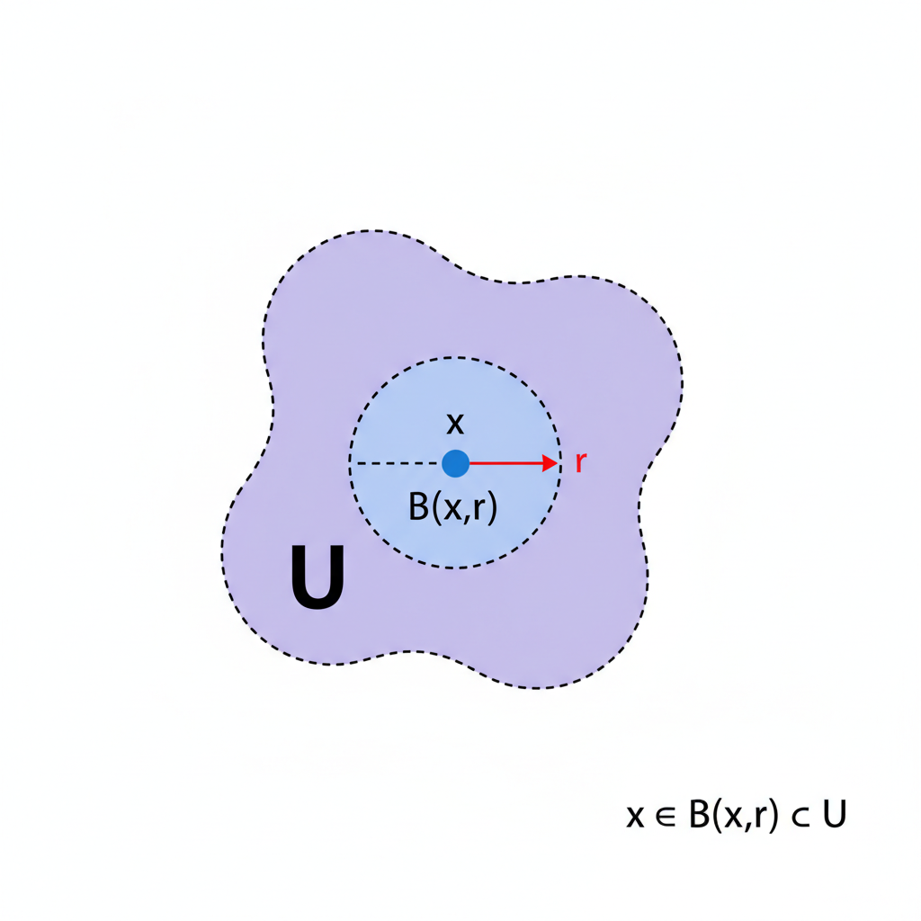
It is straightforward to verify that this family of subsets satisfies the three axioms of a topological space. This topology admits the following equivalent, more constructive description:
Remark: Throughout the rest of this course, we shall always work within a NVS or a Hilbert space. We will establish a number of sequential characterizations of topological properties (closure, continuity, density, etc.), meaning that purely topological properties will be expressed as statements about sequences. It is important to understand that these characterizations, which are often very practical, all arise from the same underlying mechanism in a NVS.
Specifically, to study the behavior of a subset or a map near a point , one exploits the availability of a countable family of nested balls whose radii tend to . Choosing a point in each ball yields a sequence converging to ; the topological property under study then translates into properties of these sequences.
This is also why the sequential characterizations stated in this lesson are specific to metric spaces—in particular to NVS and Hilbert spaces—and do not extend to general topological spaces.
3. Closed sets, closure, and dense subsets
We begin with two immediate applications of this sequential mechanism to the notions of closed set and closure. The counterpart of open sets is closed sets: a closed set is generally defined as a subset of whose complement is open. In a normed space, this definition admits a very useful sequential characterization:
In other words, a closed set is stable under taking limits: limits of sequences of elements of the closed set remain in the closed set. Given any subset of , one can augment it with all limits of sequences of elements of . This extension is called the closure of , and2 is denoted :
It follows from these two facts that a set is closed if and only if it equals its own closure : the set already contains all its limit points. We began this chapter with the open interval . One can easily construct sequences of elements of that converge to or to . Moreover, constant sequences obviously converge to . Consequently, the closure of this open set is the closed interval .
Remark: The sequential characterizations above involve the notion of convergence of a sequence, which will be formalized in the next section. For now, the reader may rely on the usual intuition: means that the approach arbitrarily closely in the sense of the norm, .
Dually to the closure, the interior of a subset is defined as the largest open set contained in , denoted . Equivalently, it is the set of points for which there exists an open ball centered at entirely contained in . An open set is its own interior.
Finally, the boundary of is the set of points that belong to the closure but not to the interior:
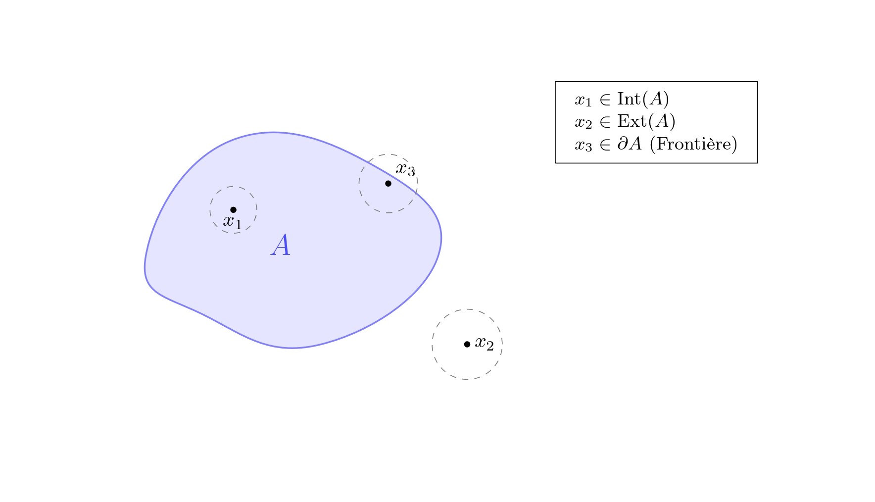
All these notions are particularly transparent in the case of the open ball of radius centered at :
- The open ball is its own interior,
- The closure of the open ball is the closed ball, denoted
- The boundary is the sphere of radius centered at , denoted
- The exterior of the open ball, defined as the interior of its complement, equals .
The density of a subset in is a notion inherited from the preceding ones.
By Theorem 1, this means that is dense in if every point of can be approximated arbitrarily closely by elements of . For example, continuous functions are dense in .
We note the following points:
- A dense subset cannot be closed, unless it equals the whole space. Indeed, if is both dense and closed, then .
- A dense subset is not in general open: it must be able to approximate elements it does not contain. For example, is dense in but is not open in : no open ball centered at a rational number is contained in . On the other hand, is a dense open subset of : so it is possible, intuitively, by removing a "small" set of points from the whole space. More precisely, the theorem states that if is a closed set with empty interior, then is a dense open set.
4. Strong and weak convergence
The sequential characterizations we have just seen all rested on the intuitive notion of convergence . It is time to formalize this. In a Hilbert space, we will moreover see that there exist two distinct notions of convergence: strong and weak.
4.1. Strong convergence of a sequence of vectors
In a NVS, a sequence converges to when its terms approach arbitrarily closely.
This is called strong convergence in reference to the strong topology, or equivalently convergence in norm. In Dirac notation, converges strongly to if and only if .
Remark: Strong convergence implies convergence of norms. Indeed, by the reverse triangle inequality3:
Thus, if strongly, then . The converse is false4. From a quantum perspective, strong convergence of physical (i.e., normalized) states with guarantees that the limiting state is also normalized, : the total probability remains equal to .
This notion of convergence may seem obvious if one restricts attention to the normed space , i.e., the usual Euclidean space. But the infinite-dimensional case is less straightforward. In a function space such as , which is a NVS and even a Hilbert space, the strong convergence just described concerns the convergence of a sequence of functions toward a limiting function .
Real analysis already provides notions of convergence for such sequences of functions, but they are not the same. On one hand, there is pointwise (or simple) convergence: converges pointwise to if for every . On the other hand, there is uniform convergence: the deviation between the sequence and its limit is controlled globally over the entire domain, i.e., . That is, for a given error tolerance , one can find a rank beyond which the entire sequence falls within a tube of width (in modulus) around the limiting function. Uniform convergence clearly implies pointwise convergence.
Where does strong convergence fit in this picture? It is different from both. It is mean-square convergence. Indeed, in this setting it is expressed via the standard inner product of , and hence via the integral of the squared modulus:
Strong convergence implies neither pointwise nor uniform convergence. Similarly, neither pointwise nor uniform convergence implies strong convergence in 5.
Let us exhibit a counterexample showing that pointwise convergence does not imply strong convergence: consider the sequence of functions on defined by a peak of width and height :
Intuitively, this is a wave function one tries to localize more and more precisely. For any , there exists large enough so that . Therefore converges pointwise to the zero function. However, computing the norm:
The norm remains constantly equal to , so the sequence cannot converge strongly to the zero function.
There is therefore a clear incompatibility between these two modes of convergence. This example shows that if pointwise convergence were the appropriate notion in quantum mechanics, one could construct sequences of wave functions converging pointwise to zero, meaning that in the limit the particle disappears (total probability zero), thereby violating the conservation of probability that is essential to the interpretation of the quantum formalism.
We will explain below how the quantum postulates actually impose the strong topology on the Hilbert space, see Section 10.
4.2. Weak convergence of a sequence of vectors
The reason we speak of strong topology and strong convergence is that a Hilbert space also admits a weak topology and a notion of weak convergence. The latter is convergence "up to an inner product":
The interpretation is as follows. The inner product represents the orthogonal projection of onto the direction . Weak convergence therefore requires each of these projections to converge. In quantum mechanics, means that each probability amplitude converges individually to for all . However, this coordinate-wise convergence does not impose strong convergence of the sequence. We have the following proposition:
Proof.
A more physically meaningful counterexample is that of probability dilution. Suppose that is an orthonormal basis of eigenstates of the Hamiltonian (for example, the energy levels of the harmonic oscillator). Consider the sequence of states:
Each term represents an equiprobable superposition of the first energy levels. As increases, this sequence converges weakly to zero. Indeed, the probability amplitude onto any fixed state is , which tends to zero as .
Yet the particle does not "disappear": the total probability, equal to the norm of the state, remains constant since . Here, the probability dilutes over an infinite number of states without ever concentrating on any of them. Since for all , the sequence does not converge strongly to the zero vector. In fact, this sequence does not converge strongly to any element of , as it is not Cauchy: the states drift apart in the Hilbert space rather than stabilizing.
The continuous analog of the previous example consists of wave functions that spread out more and more in . The Gaussians
of increasing width converge weakly to the zero function. Indeed, for any fixed , the integral tends to zero as spreads out more and more. However, they remain normalized: for all , so and the sequence does not converge strongly to zero.
All three counterexamples relied on the infinite dimension of the space. This was necessary: in finite dimension, weak convergence is equivalent to strong convergence.
The strong topology also makes the continuous (see the next section), so that the weak topology is, in infinite dimension, strictly coarser than the strong topology. It has fewer open sets, and hence more sequences converge. This is why strong convergence implies weak convergence but not conversely.
5. Cauchy sequences, completeness, and series
The two preceding notions of convergence assume that the limit is known in advance. In practice, however, one often wishes to establish convergence of a sequence without an explicit candidate for the limit. It is therefore desirable to have an intrinsic convergence criterion. This is especially useful when asking whether an infinite sum converges. This is the purpose of Cauchy sequences and the resulting notion of completeness.
5.1. Cauchy sequences and completeness
In a normed vector space , a sequence is called a Cauchy sequence if its terms become arbitrarily close to one another:
Cauchy sequences generalize the notion of strong convergence. They are precisely all sequences that could potentially converge, since every strongly convergent sequence is Cauchy: if strongly, then the terms approach and hence approach one another. By contrapositive, a sequence that is not Cauchy cannot converge strongly (this was used in the previous section). This provides a very useful criterion for showing that a sequence does not converge: it suffices to verify that its terms do not approach one another.
We thus have the formal implication , but the converse does not always hold in an arbitrary normed vector space. For this to be the case, the space must be complete, meaning it contains all the limits toward which Cauchy sequences converge.
Recall that a Hilbert space is, by definition, a complete pre-Hilbert space, see Lesson 1. Throughout the rest of this course, we will always assume we are working in a complete space. In this case, every convergent sequence is Cauchy and conversely.
5.2. Convergence of sums of vectors
A direct application of completeness concerns infinite sums of vectors, called series, which arise frequently in infinite-dimensional quantum mechanics. As with numerical series, convergence is defined via partial sums:
There are two practical criteria for establishing convergence of a series. The first method is to determine whether the series of norms itself converges.
This approach is "crude" in the sense of being overly demanding. It does not exploit possible cancellations between the terms that might stabilize the sum. The converse is therefore false: a series can converge without the sum of its individual norms () being finite. The other method is to apply the Cauchy criterion directly to the partial sums, yielding the following criterion:
The Cauchy criterion is sharper since it concerns the norm of partial sums, not the sum of norms.
Now consider the series with (which stays on the axis). It is not absolutely convergent since diverges. It nevertheless converges by the Cauchy criterion through partial cancellation of successive terms of opposite sign: factoring out , it is a classical result for real alternating series that the series converges to . Thus:
Finally, the case of the series with is particularly interesting. It is also not absolutely convergent, yet it converges to a vector in . Here, stability comes not from alternating signs but from the pairwise orthogonality of the terms. The Pythagorean theorem indeed gives, in the Cauchy criterion:
Since the tail of the series tends to , the Cauchy criterion is satisfied.
6. Continuity of maps
Before defining continuity, let us briefly recall the notion of limit in normed spaces.
6.1. Limit of a map
Note that in the case , this recovers the usual definition of the limit of a real-valued function. In that setting, the order structure also allows one to define left and right limits. This is not possible in a general normed space: a point can be approached along infinitely many paths. One therefore requires that all sequences yield the same limit for . Note also that the definition encompasses points in the closure of the domain, not just those belonging to the domain itself. This allows one to define, when it exists, a limit at the boundary of the domain, where the function is not necessarily defined. For example, this allows one to define the limit at zero of , which equals .
This notion of limit can be reformulated in terms of sequences, which is often more tractable in practice:
6.2. Continuity of a map at a point
The notion of continuity is closely related to that of limit. A map is said to be continuous at if the limit it admits is precisely .
In — form, this definition reads:
Note that continuity at is only defined for . If and admits a limit at , one can define the continuous extension of at by setting . Such an extension is unique when it exists.
A map is said to be continuous if it is continuous at every point of its domain.
6.3. The case of linear maps
When the map is linear, one more commonly speaks of a linear operator rather than a map, but the two are synonymous. We will denote it . This case is absolutely central in quantum mechanics, which is a linear theory.
The question of continuity is radically simplified in this case. The key idea is to exploit the identity to reduce the question of continuity at an arbitrary point to continuity at the origin. This yields one of the main theorems of this chapter:
- is continuous at some point
- is continuous at (note that by linearity)
- is continuous on all of
For a linear operator, continuity is therefore a global property: either it is continuous everywhere on its domain, or nowhere on it.
Proof.
: For any and , linearity gives . If , then , and by continuity at , , hence .
: Immediate.
Another major proposition of this chapter (often stated as part of the theorem above) concerns the link between continuity and boundedness of a linear map (for a general definition of bounded maps, see the next section).
Proof.
Suppose is continuous at . Applying the definition with , there exists such that implies . The idea is then to exploit linearity as a scaling. Let be nonzero. The vector satisfies , hence . By linearity, the scaling factor propagates faithfully through :
The constant works (the inequality being trivially satisfied for ).
This characterization allows one in particular to prove the following corollary:
It suffices to show that it is bounded, which follows almost immediately.
Proof.
6.4. Discontinuity and infinite dimension
In infinite dimension, a linear operator can be either continuous or discontinuous, and if it is discontinuous, it is discontinuous everywhere on its domain. This is a rather counterintuitive object. One may legitimately ask what this means, especially if one's intuition of discontinuity is limited to real-valued functions, which have "jumps" with different left and right limits. Does an everywhere-discontinuous operator have jumps everywhere? The answer is no. In fact, the nature of discontinuity in these two cases is completely different.
To understand this better, let us first negate the - formulation of continuity at :
In other words, discontinuity at zero requires the existence of a threshold such that for every radius , however small, there exists a vector in that small ball whose image "resists," i.e., does not drop below the threshold .
One might naively suppose that discontinuity arises from a fixed direction along which the action of blows up. But this is impossible: for any fixed vector , is a vector in , and its norm is necessarily finite. By linearity, taking a sufficiently small input vector makes its image arbitrarily small. Thus the action (often called the amplification) of the operator is controlled in each individual direction.
What actually happens is more subtle. It is a sequential phenomenon: in the presence of discontinuity, one can find a sequence of unit directions whose images escape to infinity. To see this, fix a threshold and choose a sequence of radii tending to zero. Discontinuity guarantees the existence of vectors (with ) such that . Setting , linearity gives:
Discontinuity thus manifests as an escape in the space of directions: no fixed direction is problematic, but one can find a sequence of directions along which the action of the operator diverges. This is why the phenomenon can only occur in infinite dimension.
Let us return to the geometric interpretation. Can one still speak of a jump? For the function from to given by
the discontinuity at is revealed by a single fixed approach path , which shows that and hence reveals a jump.
In the case of the differentiation operator near a given point , no fixed approach path reveals the discontinuity, since for any fixed direction , one has as : there is no jump along , for any function .
On the other hand, the sequence approaches through ever-changing directions: one has in the norm, but , due to the divergence noted in the example above.
Remark: In point-particle quantum mechanics, the momentum operator is represented by , and is therefore discontinuous. As a consequence, it can only be defined on a strict subdomain of . Its self-adjointness is therefore not automatic, and depends on the boundary conditions imposed on the wave functions. This will all be detailed in the following lessons.
6.5. The case of linear functionals
In the previous lesson we saw the fundamental role of linear functionals on a Hilbert space, and in particular that of continuous ones. For completeness, we now detail what these continuous functionals are. We first have the following proposition:
Proof.
Moreover, recall that the Riesz representation theorem states that the converse holds: every continuous linear functional on is of this form. The map is therefore an isometric bijection from onto its topological dual , and this is what justifies the identification of vectors (kets) with continuous linear functionals (bras).
6.6. Continuity of the inner product
The Cauchy-Schwarz inequality also yields continuity of the inner product, which is not itself a linear map in the strict sense, but rather sesquilinear: antilinear in the first argument and linear in the second. Without going into details, we ask about joint continuity in both arguments. This indeed holds: for pairs in , one has . Proof:
We used the triangle inequality, applied Cauchy-Schwarz twice, and used the fact that remains bounded to conclude convergence to zero.
Remark: As already noted in Lesson 1, the continuity of linear functionals and of the inner product expresses physically the robustness of probability amplitudes under small perturbations of states, thereby ensuring the stability of measured probabilities.
7. Topology of vector subspaces
In what follows, we will frequently work with vector subspaces of normed spaces or Hilbert spaces. When discussing their topology, we implicitly mean the induced topology: a subspace naturally inherits the norm of by restriction, and hence the notions of open set, closed set, convergence, etc. Whether these subspaces are closed or dense depends critically on dimension. We first have the following theorem:
In particular, they can never be dense, unless they coincide with the whole space (the trivial case). The case of infinite-dimensional subspaces is richer: some are closed and others are not.
Density and infinite dimension
If is infinite-dimensional, a vector subspace of can be dense without being equal to . This is a counterintuitive phenomenon, since in finite dimension a proper subspace always lacks at least one direction to fill the whole space. In infinite dimension, however, the following holds:
The proof is immediate: if were finite-dimensional, it would be closed by the preceding theorem. Since is dense, this would give , contradicting the assumption.
It is precisely because it has infinitely many directions that a subspace can "spread" throughout the whole space (be dense) without entirely filling it (without being closed).
Example: finitely supported sequences
Consider the example of , the set of finitely supported sequences. This is a subspace of , the space of square-summable sequences. The expansion of each element uses only finitely many vectors of the canonical basis , but this number is arbitrary: there is no uniform bound on the number of directions used. This is also why this subspace is closed under addition: the sum of two elements of has finite support, possibly with a larger support. Furthermore, this shows it is dense, since any point can be approximated by the sequence of elements of obtained by truncating at its -th term:
which converges strongly to as .
This subspace is therefore dense because it is free to use any available direction, in an arbitrarily large number, which allows one to approximate any point of the full space.
The family plays a dual role: it is both an algebraic basis of (every element of is a finite linear combination of the ) and a Hilbert basis of (every element of is the limit of a series involving the ).
Example: continuous functions
However, the mechanism of density is not always of the "growing finite support" type. Indeed, let denote the set of continuous functions on . This is a vector subspace of . One can show it is dense by first approximating any function by step functions, and then these by continuous functions.
Unlike the case of , however, the algebraic nature of this density remains elusive. In the first case, the density could be explained algebraically: the (algebraic) basis of contains all the vectors of the Hilbert basis , and density uses "all directions" of , with no uniform bound on the number of directions simultaneously mobilized.
For dense in , no such statement can be made. A general result7 does affirm that possesses an algebraic basis, but:
- No explicit or constructive description of it is known,
- The density is proved by analytic arguments and escapes any purely algebraic understanding.
In conclusion, dense subspaces in infinite dimension are subtle, and sometimes surprising, objects. Unlike the finite-dimensional case where a proper subspace can never be dense, infinite dimension allows this phenomenon, and it is not always possible to express it in purely algebraic terms.
In quantum mechanics, unbounded (or discontinuous) linear operators, such as the momentum operator encountered earlier, can only be defined on a proper vector subspace of . In order for them to still qualify as observables, one requires this subspace to be dense: this guarantees that no physical state is topologically inaccessible from the domain of the operator, and it is also the condition for the adjoint of the operator to be uniquely defined (see the next lesson).
8. Bounded sets
In a normed space , a subset is said to be bounded if there exists such that
Unboundedness has a sequential characterization: is not bounded if and only if there exists a sequence of elements of such that .
As seen in Section 6.3, it is the notion of bounded set that characterizes continuity of linear maps between normed spaces: a linear map is continuous if and only if it is bounded, meaning it maps every bounded subset of to a bounded subset of .
For the record, note that bounded and closed are two independent notions:
- The open ball is bounded but not closed.
- A linear line (with ) is closed but not bounded.
- The closed ball of radius is both bounded and closed.
9. Compact sets
Compactness has a purely topological definition that we will not detail here. In normed spaces it admits a sequential characterization (the Bolzano-Weierstrass theorem) that we will take as a definition:
- A subset is called compact if every sequence of elements of admits a subsequence converging to an element of .
- A subset is called precompact (or relatively compact) if its closure is compact.
A precompact set is thus nearly compact: it suffices to adjoin its limit points to make it closed and compact. A compact set is necessarily closed and bounded8. The Heine-Borel theorem tells us that the converse holds in finite dimension: a set is compact if and only if it is closed and bounded9.
We sketch the proof in finite dimension, as it explains why the converse fails in infinite dimension. On a closed interval of , given an infinite sequence of points, one can bisect the interval: at least one half contains infinitely many points. Iterating this bisection, one constructs a sequence of nested intervals whose length tends to zero and each of which contains infinitely many points of the sequence. This allows one to extract a subsequence converging to the unique point common to all these intervals.
In dimension , one generalizes this process coordinate by coordinate: one first extracts a subsequence converging in the first coordinate, then from it a further subsequence converging in the second, and so on. Since there are only finitely many directions to handle, one always ends up with a convergent subsequence, see Figure 3.
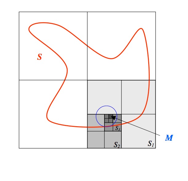
Figure taken from https://old.maa.org/press/periodicals/convergence/an-analysis-of-the-first-proofs-of-the-heine-borel-theorem-cousins-proof
In infinite dimension, boundedness allows one to apply the bisection argument detailed above, but this does not control the infinitely many directions along which points of the sequence can escape. We thus have the striking counterexample due to Riesz:
The proof is not immediate in the case of a general NVS, but is very simple in a Hilbert space. It suffices to consider the sequence of vectors of a Hilbert basis (which is orthonormal). One has for all . Since the points remain at constant mutual distance, no subsequence can be Cauchy, and hence none can converge.
The unit ball seems compact at first glance because one tends to picture it in finite dimension, but in reality it is too large in infinite dimension to be compact. In contrast, a much smaller set, such as the Hilbert cube:
is compact because it becomes arbitrarily thin in the high-index directions, which forces the existence of accumulation points.
10. The appropriate topology in quantum mechanics
All the preceding sections have prepared us for the question of the appropriate topology to use in quantum mechanics. Consider a sequence11 of physical (normalized) states converging to a limiting state . It is natural to require that experimental predictions converge consistently: measurement probabilities and mean values of observables . The question is: in what sense should the convergence be understood? That is, for which topology?
The measurement postulate states that the probability of obtaining the outcome when the system is prepared in state is given by: . For the probabilities to converge, it is therefore sufficient that the probability amplitudes converge:
which is nothing other than the weak convergence seen earlier: . Weak convergence also guarantees convergence of the mean values of bounded observables12.
The weak topology thus seems like a good candidate. But, as seen in the counterexamples from the previous sections, weak convergence is not sufficient to impose strong convergence. In particular, the norm does not necessarily converge:
In quantum mechanics, however, conservation of total probability is mandatory for the interpretation of the theory. One therefore requires convergence of the norm: , which physically means there is no probability leakage. The following theorem allows one to combine these two requirements:
We arrive at the following remarkable conclusion, which closes this lesson: the strong topology is not merely natural from a mathematical standpoint, it is imposed in quantum mechanics by the consistency of the postulates. First, because probabilities are expressed via continuous linear functionals (weak convergence), and second, because of conservation of total probability (convergence of the norm).