Lesson 1 stated the postulates of quantum mechanics without really discussing them. What do they tell us about the physical system, its state and measurement outcomes? Here we examine their consequences, their differences from the classical framework and the questions of interpretation that they raise.

1. Formulations and interpretations

Let us first note that there are formulations and interpretations of quantum mechanics other than the Copenhagen interpretation. They do not all accord the same status to the postulates presented here. One of the best-known interpretations, Everett's many-worlds interpretation, for example abandons the postulate of wave-function collapse. The global state always remains in superposition and evolves unitarily according to the Schrödinger equation. During a measurement, the different possible outcomes are then associated with “distinct branches” of this global state. The observer is in turn associated with these different outcomes: in each branch, the observer perceives a unique result, determined relative to that branch, which appears random, while the global state, “the wave function of the Universe”, still contains all the branches corresponding to all possible outcomes¹.

On the other hand, the past thirty years have seen the rise and development of quantum computing and quantum cryptography. This has greatly renewed interest in the foundations of the theory, and these efforts have in particular led to reformulations of its postulates in a form quite different from that set out in Lesson 1. In some of these approaches, the Hilbert-space structure is not postulated, but derived from a different set of axioms, informational in nature. These approaches will be discussed later in the book.

All this shows that, even today, more than a hundred years after the beginnings of quantum mechanics, we should remain open-minded about both the formulation and the interpretation of the theory. The subject is far from settled and has seen major advances in recent decades, both experimental and theoretical.

For the moment, we shall not enter into the question of interpretations. We shall simply examine the framework that we have just established. Let us begin with the first question it raises: what physical meaning should be given to the state vector?

2. The ontological problem

According to the first postulate, concerning the state space, the state of a quantum system is represented by a normalised vector, up to a global phase, belonging to an abstract Hilbert space whose dimension and structure depend on the system under study.

The state vector is therefore not a vector in “real” physical space, the space in which we live and which can locally be identified with $\R^3$. A ket cannot be “touched”, or even directly visualised in physical space. Let us compare it with a classical field. A magnetic field is admittedly not immediately visible, but its effects can be made visible, for example with iron filings arranged around a magnet. It has a definite value at each point in space, the components of which can be measured.

Even the wave function $\psi(\mathbf{x})$, which seems to “live” in $\R^3$, is only a particular representation of the ket $\ket{\psi}$: its representation in the position basis. We can equally well represent this ket in the momentum basis, as we shall see in Lesson 4; the explicit dependence on spatial position then disappears. Furthermore, the wave function cannot be determined by a single measurement. What can be done, for example, is to check for the presence or absence of the particle in a given region. By repeating this measurement many times on identically prepared systems, we obtain an approximation to the position probability density, and hence to $|\psi(\mathbf{x})|^2$. This is not sufficient, however, to determine the wave function completely, since in particular this procedure provides no information about its phase.

The problem becomes still more apparent when we consider a many-particle system. In that case, the composition postulate, introduced as the sixth postulate, will lead us to define, for $N$ bodies, not necessarily $N$ individual wave functions on $\R^3$, but a global wave function

defined on the configuration space $\R^{3N}$. In some special cases, this global function can be factorised into individual wave functions, but this is not always possible. This configuration space is not the same as our three-dimensional physical space. The question then arises with particular force: in what sense can the wave function be said to be “real”?

This difficulty is one aspect of the ontological problem of quantum mechanics: what kind of reality should be ascribed to the wave function? Without entering here into the details of the interpretations, we can identify a few broad positions. Realist views of the wave function hold that it represents an objective aspect of the physical world, independently of what an observer knows about the system. Operationalist or instrumentalist approaches emphasise its role in calculating the probabilities of experimental outcomes, without necessarily ascribing to it a physical reality of its own. Relational interpretations, for their part, view the quantum state relative to another physical system, rather than as an absolute property of the system considered in isolation. These positions do not constitute an exhaustive classification, nor are they necessarily mutually exclusive categories. We shall describe them more precisely later. For now, we need only bear in mind that knowing how to use the state vector to make predictions is not sufficient to determine what it represents physically.

3. The superposition principle.

The first postulate also contains the superposition principle through the linear structure of Hilbert space: a non-zero linear combination of state vectors, after normalisation, again defines a pure state. Such a state can therefore in principle be prepared, subject to the superselection rules mentioned below. This addition applies to the vectors that represent the states. The difference from classical physics appears when states corresponding to mutually exclusive properties are combined. Thus, one is tempted to say that a spin can be both up and down, and a cat both alive and dead.

Care is needed, however, in using the verb “to be”, as Niels Bohr taught us, precisely because the reality of the wave function is open to debate: is the cat really in a superposition? From the Bohr perspective presented here, this question has no meaning independently of the measurement conditions that give physical content to the properties under discussion. To express this idea figuratively, “being only becomes being” when a measurement is performed: it is then that a definite property, expressed in classical language, can be ascribed to the system. In the case of the cat, one obtains one of two classical and mutually exclusive outcomes: either alive or dead. It is therefore the physical meaning of the verb “to be” that is at issue, not the possibility of writing a superposition. Nevertheless, the mathematical description of the system as a superposition is correct within the model and allows verifiable predictions to be made, in particular the calculation of probabilities.

Let us examine the consequences of these superpositions for position and energy.

Superpositions and delocalisation.

In the quantum mechanics of a point particle, spatial delocalisation is generic. The wave function introduced in Lesson 1 describes a single state of the particle by amplitudes distributed in space. According to the probability rules already stated, the particle can therefore be detected in different regions of space. It does not have a precise position in the classical sense, but a “probability cloud”, as it is called, which can be more or less extended.

Care must be taken, however, not to generalise the image of a cloud in our space too quickly. As explained above, for $N$ particles, the wave function depends on an entire configuration, that is, on the positions of the $N$ particles: it is defined on $\R^{3N}$. This does not mean that the particles move in a $3N$-dimensional physical space! Each moves in our three-dimensional space, but $3N$ coordinates are needed to describe their positions together. The probabilities then concern questions such as “particle 1 is in region $R_1$, particle 2 in region $R_2$, and so on”. We shall make this formalism more precise with composite systems.

This delocalisation must not be confused with the non-locality of quantum mechanics, which concerns correlations between distant systems. Simply writing a wave function on $\R^{3N}$ is not sufficient to establish this non-locality. We shall return to it with Bell experiments.

Superpositions and energy.

As we saw in Lesson 1, the Hamiltonian governs time evolution. Let us consider here the case of a discrete spectrum and a time-independent Hamiltonian: a state can be written in an energy eigenbasis as $\kpsi = \sum_n c_n \ket{E_n}$. As soon as several distinct energies contribute to this superposition, the energy does not have a definite value.

Energy conservation then takes a probabilistic form: as established in Lesson 1, the distribution of possible energies remains constant, and hence so does their mean. This does not prevent the state from evolving: the relative phases between components of different energies vary and can produce temporal interference, such as the quantum beats studied in Lesson 11. An energy eigenstate, by contrast, remains stationary: only its global phase changes, without changing the measurement probabilities of a fixed observable.

In conclusion, all superpositions are therefore possible, and sometimes even necessary²: nothing in the postulates rules out any superposition of states a priori.

4. Quantisation and spectra

The second postulate contains the “quantisation principle”: some physical quantities can take only discrete values. Moreover, these discrete values can be calculated by finding the spectrum, which makes this postulate a means of formulating verifiable predictions, provided that we know which observable $\hat{A}$ is associated with a given physical quantity measurable in the laboratory (cf. the canonical quantisation procedure at the end of this lesson).

A particularly important case is energy: the observable is then the Hamiltonian $\hat H$, and its discrete eigenvalues give the energy levels of the system. For an atom, the differences between these levels determine the frequencies of the absorption and emission lines associated with the allowed transitions, according to $h\nu = |E_m-E_n|$. We thus pass from calculating the spectrum of $\hat H$ to the lines observed in the laboratory. Explaining these lines and predicting their positions was one of the great successes of early quantum mechanics.

Ironically, this quantisation is not a general principle, even though it gave the theory its name. Admittedly, in finite dimension, all observables necessarily have a discrete spectrum, and thus all quantities measurable on a system will indeed be quantised. But in infinite dimension, some observables have a discrete spectrum and others, such as the position operator, have a continuous spectrum. The Hamiltonian itself, depending on the system under study, may have a discrete spectrum, a continuous spectrum, or both parts (for example, continuous for a free particle on $\R$, but discrete for the same particle in an infinite well of finite width).

In finite dimension, finding the eigenstates amounts to diagonalising a self-adjoint matrix. The method is that of linear algebra: we find the eigenvalues using the characteristic polynomial, then the associated eigenvectors. In simple examples, these calculations can be carried out by hand, particularly when the matrix has low dimension or decomposes into blocks. When usable analytical expressions are not available, numerical diagonalisation can be used to calculate approximate values and deduce predictions from them, while controlling the precision of the calculation.

In infinite dimension, the solution methods change, but the objective remains the same: to diagonalise the operator, that is, to determine its spectral decomposition, whether the spectrum is discrete or continuous. For the energy eigenstates of a particle, for example, one must solve $\hat H\psi = E\psi$. The unknown is now a function, and the Hamiltonian involves its derivatives: the same eigenvalue equation therefore takes the form of a differential equation rather than a matrix problem. The conditions imposed on the wave function, which select the admissible energies, must also be taken into account; solving the equation without considering them is not sufficient.

Potential wells, the harmonic oscillator and the hydrogen atom are models for which this calculation can be carried out explicitly. But the difficulty grows rapidly: in the helium atom, the two electrons interact, and the complete problem can no longer be solved in the same way as for the single electron of hydrogen. Approximations or numerical calculations are required. With more electrons and several nuclei, we enter the domain of quantum chemistry. The simple examples that we are about to study therefore also serve to teach us the methods we shall need to tackle more complex systems.

5. Compatible and incompatible observables.

After seeking to diagonalise one observable, we can ask whether two observables can be diagonalised in the same basis. An important theorem answers this question: the simultaneous diagonalisation theorem, encountered in Lesson 6 of Theme 2. Standard in finite dimension, it generalises to infinite dimension subject to certain precautions, mentioned below. Let us begin in finite dimension: if two observables commute, $[\hat{A}, \hat{B}] = 0$, then there exists an orthonormal basis of common eigenvectors of $\hat{A}$ and $\hat{B}$.

What does this result mean physically? A vector in this basis represents a state in which the two quantities each have a definite value. It may be denoted by $\ket{a_i, b_j}$: a measurement of $\hat A$ gives $a_i$ with certainty, and a measurement of $\hat B$ gives $b_j$ with certainty. The two labels therefore denote one and the same state, which is an eigenstate of both observables. It is in this sense that these observables are said to be compatible.

Conversely, if two observables do not commute, then a basis of common eigenvectors does not exist: some eigenvectors may be common, but they do not form a complete common basis. This has consequences for successive measurements: measuring $\hat B$ may alter the probabilities of the outcomes of a subsequent measurement of $\hat A$.

Consider, for example, a sequence of three measurements: $\hat{A}$, then $\hat{B}$, then $\hat{A}$ again. One may then obtain successively $a_i$, $b_j$, then $a_k \neq a_i$, which illustrates the following point: when $\hat{A}$ and $\hat{B}$ do not commute, measuring $\hat{B}$ may alter the predictions based on the information acquired in the first measurement of $\hat{A}$. This result follows from Postulate 3, wave-function collapse: after each measurement, the system is projected into the eigenstate corresponding to the outcome obtained. Thus, in the non-degenerate case, after the second measurement the system is in the state $\ket{b_j}$, which may not be an eigenvector of $\hat{A}$ and can therefore be written as a linear combination of eigenstates of $\hat{A}$. Consequently, according to Postulate 4, the third measurement has a non-trivial probability distribution over the eigenvalues $a_k$ of $\hat{A}$, allowing an outcome different from that of the first measurement.

We already encountered this situation in Theme 1, Lesson 1, and repeated the calculation in Lesson 2: in the Stern—Gerlach $z-x-z$ sequence, after selecting $z+$ and then $x+$, the last measurement gives $z+$ or $z-$ with equal probability. The observables along $z$ and $x$ do not commute: they are incompatible.

In infinite dimension, the general compatibility of two observables is formulated in terms of the commutation of their spectral projectors. The vanishing of a formal commutator on a common domain is not always sufficient. The matrix examples avoid this difficulty.

6. Uncertainty relations

The non-commutation of observables also enters into uncertainty relations. Heisenberg's relation for position and momentum is one example; we shall establish a general form for two observables $\hat A$ and $\hat B$.

These relations are often presented as a limit on the precision with which two physical quantities can be known “simultaneously”. But the word “simultaneously” can be misleading, suggesting that temporality is involved. It is not a matter of performing two measurements at the same instant, or of choosing their order: the question is whether a single quantum state can assign well-defined values to both quantities. Thus we return to simultaneous diagonalisation: having two certain values requires a common eigenstate of the two observables. If they do not commute, an entire basis of such states cannot be constructed, even though some common eigenstates may exist. Uncertainty relations quantify the constraints on the dispersions in a single prepared state.

To give this question a concrete meaning, consider the following experimental procedure:

1. Prepare a large number of identical systems in the same quantum state $\ket\psi$.
2. On one half, measure $\hat A$. The results allow an estimate of a mean and a standard deviation $\sigma_{A}$.
3. On the other half, measure $\hat B$. In the same way, estimate the mean and the standard deviation $\sigma_{B}$ of this second distribution.

A small standard deviation means that the results are concentrated around their mean; a large standard deviation indicates that they are more dispersed. This is the dispersion predicted by the Born rule, which may remain even with an ideal apparatus. The two measurements concern different systems: the first therefore does not disturb the second.

The formalism imposes a bound on the product $\sigma_{A}\,\sigma_{B}$ of these two dispersions. If this bound is strictly positive, the two distributions cannot both be arbitrarily narrow. Within the formalism set out by the postulates, this relation is a theorem:

The bound depends on the state. A non-zero commutator does not mean that its expectation value is non-zero in every state. For an arbitrary pair, one should therefore not conclude that every reduction in $\sigma_{A}$ always forces $\sigma_{B}$ to increase. The situation is special for position and momentum: the commutator is $[\hat X,\hat P]=i\hbar\mathbf{1}$ on the appropriate domain, which gives $\sigma_{X}\,\sigma_{P}\geq\hbar/2$. This Heisenberg relation is also written as $\Delta x\,\Delta p\geq\hbar/2$, where $\Delta x$ and $\Delta p$ denote the same standard deviations. If a state is prepared whose position distribution is very narrow, its momentum distribution must therefore be sufficiently broad to satisfy this bound. We shall return to the position—momentum commutator at the end of the lesson, and then to its concrete realisation in Lesson 4.

If the real part is also retained in the proof, one obtains the Robertson—Schrödinger inequality:

The braces denote the anticommutator $\hat C\hat D+\hat D\hat C$. This form additionally contains a covariance. The preceding version will suffice for our first applications.

The relation is not a general formula for the error of an apparatus or for the disturbance caused by a first measurement. These questions are related but distinct. Similarly, since time is a parameter here rather than an ordinary observable, an expression $\sigma_{E}\,\Delta t$ must be accompanied by a precise definition of $\Delta t$.

7. Continuous evolution versus quantum jumps

Outside a “measurement”, a quantum state evolves according to the Schrödinger equation, equivalently under the action of the unitary evolution operator $U(t,t_0)$, as discussed in Lesson 1. In particular, under this action, the path traced by $\ket{\psi(t)}$ is (strongly) continuous in Hilbert space. Moreover, the evolution is linear: if $\ket{\psi(t)} = U(t, t_0)\ket{\psi(t_0)}$ and $\ket{\phi(t)} = U(t, t_0)\ket{\phi(t_0)}$, then by linearity:

Finally, unitarity means in particular that, knowing $U$ and $\ket{\psi(t)}$, one can recover the initial state, since $U$ is invertible: $\ket{\psi(t_0)} = U(t, t_0)^{-1} \ket{\psi(t)}$. In other words, this evolution is reversible (no information is lost).

By contrast, during a measurement, the pre-measurement ket must be projected and renormalised onto the eigenspace associated with the value obtained. This operation is modelled as a “quantum jump”: within the measurement postulate, the transition is considered instantaneous, and the path of the ket appears discontinuous in $\mathcal{H}$. The need to renormalise the state makes this operation non-linear (we do not merely project; we also renormalise). Finally, it is generally a non-unitary operation because it is not injective: all initial states of the form $\ket{\psi} = c_n \ket{a_n} + \sum_{m \neq n} c_m \ket{a_m}$ (with $c_n \neq 0$) can lead to the same measurement outcome $a_n$, and hence to the same final state $\ket{a_n}$ after collapse. The infinity of possible initial states “collapses” to a single final state, and observing $a_n$ does not reveal what the initial state was before the measurement. The collapse model describes a discontinuous, non-linear and irreversible evolution (information about the initial state has been lost).

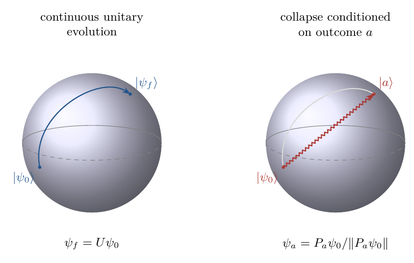
The measurement postulate and Schrödinger evolution thus describe two distinct regimes of evolution. In the formulation presented here, unitary, reversible evolution is interrupted during a measurement by a collapse conditioned on the outcome obtained. This collapse is not deduced from the Schrödinger equation: it is the subject of a separate postulate.

Is the formalism itself inconsistent? Not immediately: the Schrödinger evolution postulate as we stated it concerns an isolated system, whereas a measurement involves an interaction with an apparatus; the measured system is therefore not isolated. This distinction is not sufficient to resolve the difficulty, however, since the apparatus can be included in a larger system. Can the measurement postulate then be derived from a linear, continuous and unitary evolution of the composite system {system + pointer + environment}? By pointer, we mean the part of the apparatus whose state allows the outcome to be read; the environment comprises the other degrees of freedom of the apparatus and the surroundings (air, photons, and so on).

Decoherence theory studies one aspect of this question: how interaction and entanglement with the environment suppress interference observable in the system alone, while the global evolution remains unitary. This suppression is not sufficient, by itself, to select a unique outcome. Its theoretical developments are associated in particular with H. Dieter Zeh^[2] and Wojciech H. Zurek^[3]. Experiments have subsequently made it possible to track this loss of coherence, notably in work by the teams led by Serge Haroche on cavity fields^[4] and David Wineland on trapped ions^[5]. We shall study these mechanisms after developing the formalism of composite systems.

Several questions remain to be distinguished. Is a quantum jump instantaneous? And if not, how long does a measurement take? Since our description alternates between Schrödinger evolution and state collapse, what determines that a measurement takes place at that precise instant? In other words, what criterion makes us pass from one evolution rule to the other?

Alongside this question of the time of measurement is that of the boundary between the two descriptions. The Heisenberg cut is the separation between the part of the experiment described quantum mechanically and the apparatus whose readings are described classically^[7]. The postulates presented here do not set a threshold of size or mass that would automatically place this boundary. If the apparatus is included in the quantum description, one must then ask how a definite reading is to be accounted for. It is this difficulty that the following thought experiments bring to light.

8. The measurement problem

The difficulty concerns in particular the individual outcome: how can one account for the fact that a measurement gives a definite outcome if the system and apparatus together are described by unitary evolution?

The composition postulate already allows the difficulty to be formulated precisely. Let a system initially be in the state $\alpha\ket0+\beta\ket1$ and a second system, serving as apparatus or observer, in a state $\ket{M_{\text{ready}}}$. An interaction that unambiguously correlates the two outcomes with the two corresponding readings would lead, by linearity, to

Schrödinger evolution thus produces an entangled superposition of the composite system; it selects neither of the two terms.

In the Schrödinger's cat thought experiment, the states $\ket{M_0}$ and $\ket{M_1}$ represent, at the end of a chain of macroscopic amplification, a live cat and a dead cat. The question is not simply to declare the cat to be “in two classical states at once”, but to understand why the linear evolution of the global system does not by itself lead to the single outcome observed by an observer.

Wigner's friend makes the tension still clearer. For the friend enclosed in the laboratory, a definite outcome has been observed and the collapse postulate leads the friend to assign the corresponding state. Wigner, on the other hand, if he treats the entire laboratory as an isolated system, still assigns to it the preceding entangled superposition. At what point should collapse occur, and can the two descriptions be simultaneously consistent? The formalism presented so far poses the question clearly, but does not yet answer it.

We shall return to these thought experiments after a detailed study of composite systems.

9. The correspondence principle and the question of the classical world

We have emphasised the differences between the quantum postulates and the classical description. One question nevertheless remains: if the objects around us are made up of quantum systems, why can we so often describe them in terms of positions, trajectories and classical laws? A quantum theory must also account for situations in which classical mechanics provides experimentally verified predictions.

This requirement extends Bohr's correspondence principle. In its historical context, it related quantum transitions in particular to the components of classical motion, with asymptotic agreement at large quantum numbers^[6]. Here we shall retain the following more general requirement: in regimes where the classical description is valid, quantum predictions must reproduce it to the precision under consideration. This principle guides the construction of models; by itself, it does not provide a prescription for choosing all their operators.

The question of the emergence of the classical world then asks how this agreement is achieved. The prepared states, observation scales and timescales under consideration must be specified. Recovering a classical law for certain expectation values is not necessarily enough to describe a localised object following a trajectory: the dispersions and their evolution also matter. The role of the environment, mentioned above in connection with decoherence, enters into this discussion, as does the justification for the classical description of the apparatus beyond the Heisenberg cut. We leave it open at this stage: the postulates introduced do not yet provide an explanation of all these phenomena, even though certain mechanisms can be studied in specific models.

To proceed, let us therefore distinguish two approaches: constructing a quantum model compatible with known physical constraints, and then studying the conditions under which this model recovers classical behaviour. Let us begin with the first, using the example of a particle.

10. Constructing a quantum model

The postulates define a common framework. To describe a specific system, its degrees of freedom, a Hilbert space, the observables and a Hamiltonian must still be chosen. Just as Newton's laws must be supplemented by a model of the forces, the quantum postulates alone do not determine these objects.

Experiments, symmetries and the correspondence requirement guide their choice. When a classical model is available, canonical quantisation provides a method of construction. We shall apply it to a non-relativistic spinless particle on a line, in a real time-independent potential: starting from the classical Lagrangian, identifying the momentum and Hamiltonian, then choosing the quantum observables and their commutation relations.

10.1. The classical starting point

For a particle of mass $m$ in a potential $V(x)$, the Lagrangian is

The Euler—Lagrange equation gives $m\ddot x=-V'(x)$. The canonical momentum conjugate to $x$ and the Hamiltonian are

Hamilton's equations are then

These relations will guide the construction of the quantum model. The classical Hamiltonian $H_{\mathrm{cl}}$ is a function of two variables; the quantum Hamiltonian $\hat H$ will be an operator.

10.2. Canonical quantisation

In the model adopted, the position observable $\hat X$ and momentum observable $\hat P$ obey the canonical commutation relation. The Hamiltonian is also chosen so as to retain the form of the classical energy:

The commutator means $\hat X\hat P-\hat P\hat X$. The equality applies to states on which these two products are defined. In the following lesson we shall construct a concrete representation and verify this relation by an explicit calculation.

This prescription defines the non-relativistic model under study. It is not a consequence of the postulates of Lesson 1 alone. Symmetries, observations and correspondence with classical mechanics guide the choice. For more general classical expressions containing products of $x$ and $p$, operator ordering may become an additional question.

10.3. Commutator and correspondence

We can now return to the correspondence requirement, with the objects needed to give it precise content. The general principle presented above does not by itself fix the commutator. We shall impose a stronger condition: an exact relation for the evolution of expectation values, valid for all admissible states and for a family of potentials. The Ehrenfest theorem of Lesson 1 will then allow us to derive a constraint on $\hat X$ and $\hat P$.

We have thus fixed the algebraic prescription. It remains to construct a state space and operators that realise it: we shall move to the position representation in the following lesson.

11. References