Lesson 6: Potential wells and tunnelling
Keywords : Potential wells, Boundary conditions, Bound states, Reflection and transmission, Tunnelling
We now know how to write the Schrödinger equation for a particle, and we saw in the previous lesson that solving the dynamics amounts to finding the stationary states, that is, solving the eigenvalue equation
In this lesson, we shall solve it explicitly for piecewise constant potentials: wells, steps and barriers. These models are of course idealisations, since no real potential has discontinuities. But they have two major advantages. First, the potential is constant on each interval and we already know the solutions: oscillatory, exponential or affine depending on the sign of (see Lesson 5). All the physics then lies at the matching points, and the calculations can be carried out entirely by hand. Second, they suffice to reveal the two most striking phenomena of the quantum mechanics of a point particle: the quantisation of energy for bound states, and tunnelling, that is, the possibility of crossing a barrier that is classically impassable.
We shall first work in one dimension, with a particle of constant mass and a time-independent potential. We shall begin by setting out the rules: normalisation, matching conditions and boundary conditions. We shall then study the bound states of two wells, one infinite and one finite, followed by scattering states at a step and a barrier. We shall finish by extending the discussion to three dimensions.
1. The general method
1.1. Bound states and scattering states
Let us first recall what classical mechanics would say. A particle with energy can only be found in regions where , since its kinetic energy must be positive. If these regions are bounded, the particle is trapped and oscillates between two turning points: its motion is bound. If they extend to infinity, the particle arrives from far away, interacts with the potential and returns to infinity: this is scattering motion.
The same distinction appears in quantum mechanics, with two kinds of stationary state of very different nature.
- Bound states are normalisable eigenfunctions of , genuine vectors in Hilbert space. Their probability density is concentrated in the region of the well and decays at infinity. We shall see that the normalisability condition is satisfied only for certain values of the energy: the bound-state spectrum is discrete.
- Scattering states are generalised eigenstates, like the plane waves of the free particle. They oscillate out to infinity and are not normalisable; they exist for a continuum of energies. They do not themselves represent physical states, but rather components of normalisable wave packets, and are interpreted using the probability current introduced in Lesson 5.
1.2. The normalisation condition
For a bound state, the wavefunction must be square-integrable over the whole real line. This condition, though seemingly innocuous, is in fact highly restrictive. Suppose, for example, that in a region where , the general solution of the stationary equation is with . If , the growing exponential dominates and
A bound state must therefore have : on the right, only the decaying exponential is allowed. On the left, by contrast, it is that diverges as and must be excluded. These exclusions, combined with the matching conditions, will select the allowed energies.
For scattering states, the situation is different. A plane wave is not normalisable, but it is bounded, and a superposition of plane waves with neighbouring energies forms a normalisable packet. We therefore impose no normalisation on such a state; we fix the amplitude of the incident wave arbitrarily, and calculate the ratios of the reflected and transmitted currents to the incident current. A solution that grows exponentially at infinity is still excluded, however, because no finite-probability packet could contain it.
1.3. The matching conditions
On each interval where the potential is constant, we know how to write the general solution, which depends on two constants. We still need to know how to join these pieces at the points where the potential jumps. The stationary equation itself provides the answer.
- On an interval where is continuous, is twice continuously differentiable.
- At a point where has a finite jump, the wavefunction and its derivative are continuous: (1)
- If a point interaction is added to the potential, the wavefunction remains continuous, but its derivative has a jump: (2)
Proof.
On an interval where is continuous, the right-hand side is continuous as soon as is, and the Picard—Lindelöf theorem guarantees the existence of solutions of class . This proves the first point.
Now consider a point where jumps, and integrate the equation between and , with small. The left-hand side can be integrated exactly, giving
If and remain bounded in a neighbourhood of , the integral is of a bounded function over an interval of length : it tends to zero as . The derivative is therefore continuous at , and hence so is the function itself, which proves the second point. Note, however, that inherits the jump in : the wavefunction is only of class at the matching point.
In the presence of the term , the integral also contains the contribution , which does not tend to zero: this is the stated jump in the derivative. The function remains continuous, since if it had a jump, its derivative would contain a term and its second derivative a term, which nothing in the equation could cancel.
These rules apply to a finite jump in the potential. A point interaction in produces a jump in the derivative, while an infinite wall, which we shall now consider, requires a different condition again. Continuity of must therefore not be applied mechanically to every potential.
1.4. Infinite walls and Dirichlet conditions
A well with infinite walls models a particle perfectly confined to an interval, for example . It may be viewed as the limit of a finite well whose depth tends to infinity: we shall see below that the wavefunction penetrates into the classically forbidden regions over a length which tends to zero in this limit. The particle therefore cannot be found outside, the wavefunction vanishes there, and continuity of requires it to vanish at the boundaries:
These are called homogeneous Dirichlet conditions. The derivative , however, is not continuous at the walls: it generally takes a non-zero value just inside and is zero outside. Imposing as well would be an error, leaving no non-zero solution.
More formally, the model takes the state space to be and the Hamiltonian to be the operator acting on functions satisfying (3). It is precisely these conditions that make the boundary terms vanish in integrations by parts and render the Hamiltonian self-adjoint: on a bounded interval, the boundary conditions are part of the definition of the observable.
2. The infinite square well
2.1. The spectrum
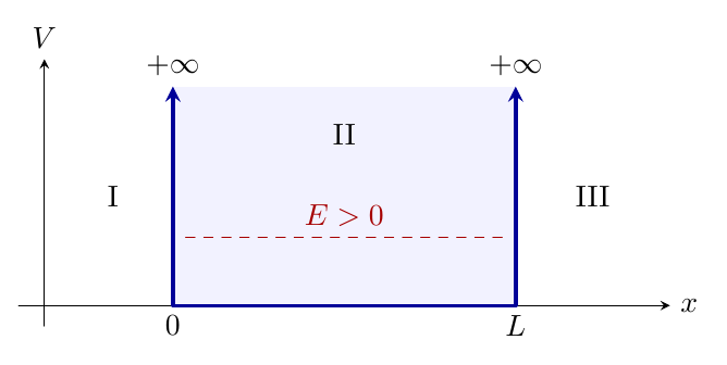
Consider a particle free to move between two infinite walls placed at and , with zero potential inside (Figure 1). This is the simplest model of a confined particle.
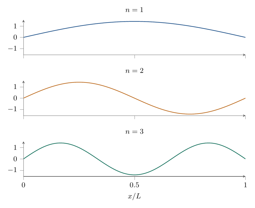
These functions form a Hilbert basis of .
Proof.
The boundary term vanishes because of the Dirichlet conditions, leaving . If , the equation would give , and the conditions would imply . Since the zero vector is not a state, we indeed have .
Set . Inside the well, the stationary equation becomes , whose general solution is
The condition at imposes . The condition at then imposes . Since for a non-zero state, we must have
Negative integers give nothing new, since they reproduce the same functions up to a sign, and gives the zero function. With , we obtain the stated energies. Normalisation follows from
which gives ; we choose to be real and positive, since the overall phase is immaterial. The orthogonality of two functions and with may be checked by writing the product of sines as a difference of cosines, but it also follows directly from the fact that they are eigenvectors of a self-adjoint operator associated with distinct eigenvalues. Finally, completeness of the family is the completeness of Fourier sine series on , a result from analysis which we shall assume.
2.2. Comments
The origin of quantisation.
The energy can take only the discrete values It is important to see where this quantisation comes from: the boundary conditions leave only the standing waves for which an integer number of half-wavelengths fits inside the well, as for a vibrating string fixed at both ends. The free particle on the whole real line, which is subject to no such condition, instead had a continuous spectrum. As we noted in Lesson 3, quantisation is therefore not a general property of quantum mechanics, but a consequence of confinement.
Zero-point energy.
The ground level has energy : the particle cannot be at rest at the bottom of the well. This can be understood from Heisenberg's uncertainty relation. Confined to the interval , the particle has a position spread at most of order , and hence a momentum spread at least of order . Since in a real state, the mean energy satisfies
This rough estimate gives the correct order of magnitude and the correct dependence on and ; the exact calculation simply replaces the factor by . Confinement has a kinetic-energy cost, which increases as when the well is narrowed. For an electron in a nm well, one finds eV, which is the order of magnitude of the energies involved in semiconductor nanostructures.
Nodes.
The function vanishes times inside the well. The higher the energy, the more the wavefunction oscillates, consistent with the fact that kinetic energy is related to the curvature of the wavefunction: indeed, from the calculation in the proof. We shall encounter this node rule again for the finite well, the harmonic oscillator and the hydrogen atom.
The dynamics.
An arbitrary state can be expanded in the basis of the , and evolves according to
The probabilities of the different energies are constant, but the position density generally depends on time because of the cross terms between levels.
Since is positive on the left half of the well and negative on the right half, the probability moves periodically from one side to the other. To quantify this, let us calculate the mean position. By symmetry, , and, writing the product of sines as a difference of cosines and then integrating by parts,
It follows that
The particle oscillates in the well at the angular frequency , set by the difference between the two energies. We shall study this type of beating in general in Lesson 11.
2.3. A delta function at the centre of the well
To see the jump condition (2) at work, add a repulsive point interaction , with , at the centre of the well (Figure 3). This term models a very thin, very high barrier with integral ; the coefficient has the dimensions of energy times length.
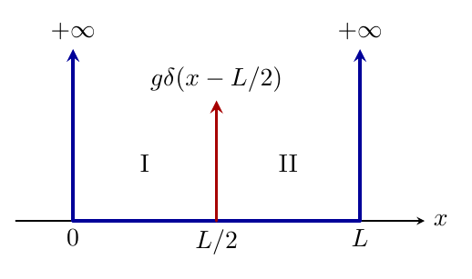
On either side of the centre, the potential is zero and the solution is sinusoidal. Choosing from the outset solutions that vanish at the walls, we write
with . It remains to impose continuity of and the jump in its derivative at . Since the potential is symmetric about the centre, we can seek separately solutions that are odd and even about this point (we shall justify this procedure below).
The solutions that are odd about the centre vanish there. The right-hand side of (2) is then zero: the delta function does not see them. These are the functions of the ordinary well, that is, the with even index , with the same energies.
For the even solutions, take . The derivative is immediately to the left of the centre and immediately to its right. The jump condition reads
This is a transcendental equation, to be solved graphically or numerically. Its two limiting cases are instructive. For , we recover , that is, the with odd index in the ordinary well. For , the right-hand side is negative and each solution is shifted towards a larger value of : the energies of the even states increase, as expected since the barrier is repulsive and these states have non-zero amplitude at the centre. As , we must have , that is, : each even state approaches the energy of its neighbouring odd state. We then obtain two independent wells of width , whose levels are doubly degenerate. For large but finite , the levels remain grouped in closely spaced pairs: this is our first encounter with the two-site model coupled by tunnelling, which we shall revisit in Lesson 11.
3. The finite square well
3.1. Solutions in the three regions
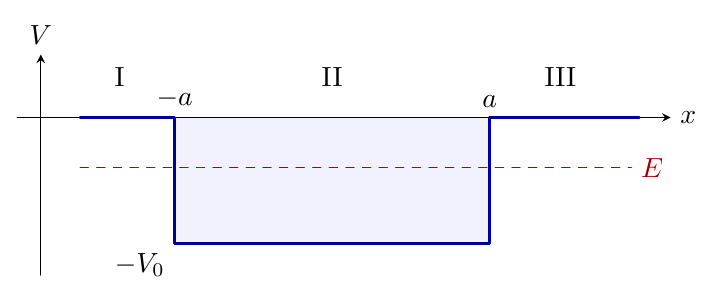
Now consider a well of finite depth and width :
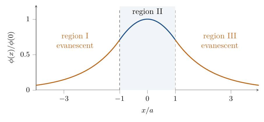
This model is more realistic than the infinite well: the particle can escape if its energy is high enough. Here we seek bound states with energy (Figure 4).
Why this range of energies? On the one hand, for , the outer regions are classically allowed and the solutions there are oscillatory (or affine if ): they are not square-integrable and describe scattering states. On the other hand, the energy of a normalised state cannot fall below the minimum of the potential, since and . We therefore set
The wavenumber describes the oscillation inside the well, where the classical kinetic energy is , and the decay outside. They are not independent, since
In region II, the equation is ; in regions I and III, it is . The normalisation condition excludes the exponential on the left and on the right. This leaves
The shifts and in the exponentials do not change the form of the solutions: they merely simplify the values at the boundaries, which are and .
3.2. Matching conditions and parity
The potential has only finite jumps: the function and its derivative are continuous at and . This gives four linear equations for the four constants :
We could solve this system directly by requiring its determinant to vanish for a non-zero solution to exist. But the calculation can be simplified considerably by using the symmetry of the problem. The potential is even, : if is a solution with energy , then so is , and hence so are the combinations , which are respectively even and odd. We may therefore seek the eigenstates among even functions (, ) and odd functions (, ), without losing any eigenvalue.
and those of the odd bound states by
where and are related by (5).
Proof.
For an odd state, and . Continuity of the derivative at gives , hence .
The corresponding wavefunctions are, up to a normalisation constant,
The normalisation must take all three regions into account. For the even state, for example, the condition reads
and similarly, for the odd state, we obtain
3.3. Graphical solution
The equations in Proposition 1 are transcendental: their solutions cannot be expressed in terms of elementary functions. The problem is nevertheless solved exactly, in the sense that the energies are the roots of explicit equations, which can be calculated numerically to any desired accuracy. To visualise these roots, introduce the dimensionless variables
The parameter measures both the depth and the width of the well. From (5), , and the equations become
The solutions are the intersections of the quarter-circle with the positive branches of the curves and , shown in Figure 6.
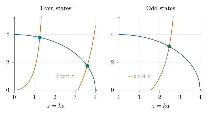
Several conclusions can be read directly from this figure.
- There is always at least one bound state. On the interval , the function starts at zero and increases, while starts at and decreases: the two curves must intersect. Thus, in one dimension, an attractive well has at least one even bound state, however shallow or narrow it may be1. Note 1: This result is specific to one dimension. In three dimensions, a spherical well that is too weak has no bound state, as may be checked later.
- The number of bound states is finite, and is , where denotes the integer part. Indeed, the positive branches of and occupy in turn the intervals , , , and so on. On each of them, the trigonometric function starts at zero and increases, while the quarter-circle decreases until it vanishes at : each interval that begins before therefore contains exactly one intersection. For , there are indeed three states. A wider or deeper well contains more.
- Even and odd states alternate as the energy increases, and the th state has nodes, as in the infinite well.
- The infinite well is recovered when . In this limit , the quarter-circle intersects the branches near their asymptotes , that is, . The energies measured from the bottom of the well therefore tend to , those of the infinite well of width .
3.4. Penetration into the forbidden region
Unlike in the infinite well, the wavefunction does not vanish at the boundary of the well: it extends into the classically forbidden regions as a decaying exponential, called an evanescent wave. This name describes the spatial dependence of the amplitude, not a decrease in probability over time: the state is stationary. The amplitude decays over the characteristic length , and the probability density as at a distance from the boundary. As the energy approaches zero from below, and the tail extends farther and farther.
The probability of finding the particle outside the well is therefore non-zero. For the even state, it is
This is a purely quantum effect: a classical particle with energy could never reach the region . This does not mean that the particle escapes: the density is stationary and the probability current is zero everywhere, since the wavefunction is real. The particle remains bound, but its wavefunction “spills out” of the well. As we shall see, it is this spillover that makes it possible to cross a barrier of finite width.
Finally, note that the bound states do not form a basis of : to describe an arbitrary state, the scattering states with energy must be added. Here the spectrum of the Hamiltonian has a finite discrete part and a continuous part.
4. Parity and non-degeneracy
We used the parity of the potential to seek even or odd solutions. This procedure has a general justification: the parity operator commutes with the Hamiltonian whenever is even, and and , whose eigenvalues are , can therefore be diagonalised simultaneously. But we obtained a stronger result: every bound state is automatically even or odd. This follows from the next result.
Proof.
The Wronskian is therefore constant on each interval where is regular, and is continuous at the matching points since , and their derivatives are continuous there. It is thus constant over the whole real line. For bound states, the functions and their derivatives tend to zero at infinity, so this constant is zero. Wherever does not vanish, may be written , hence on that interval. Uniqueness of solutions to the differential equation for given initial conditions at one point then extends the proportionality to the whole real line.
If is even and is a bound state, is a bound state with the same energy, so . Applying this relation twice gives : the state is even or odd.
The assumptions matter. A particle on a ring, whose wavefunction must be periodic and does not tend to zero, has states of the same energy with opposite momenta, . And we shall see at the end of this lesson that degeneracies are common in three dimensions.
5. The potential step
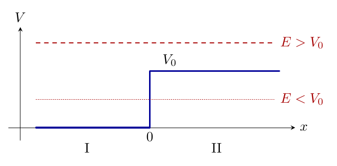
We now turn to scattering states, beginning with the potential step: for and for (Figure 7). A particle approaches from the left with energy . Classically, the situation is simple: if , the particle crosses the step and slows down; if , it bounces back. Let us see what quantum mechanics says.
5.1. Above the step
For , the solutions are oscillatory on both sides, with wavenumbers
On the left, there is the incident wave , whose amplitude we set to one, and a possible reflected wave . On the right, there is only a transmitted wave travelling to the right: a term in would describe a wave arriving from , which is not the situation under study. We therefore write
Continuity of and at gives
Substituting the first equation into the second gives , hence
These coefficients are amplitudes. To obtain reflection and transmission probabilities, the probability fluxes must be compared, and this is where the current from Lesson 5 becomes essential.
Proof.
We define and , which gives the stated expressions. Their sum is .
The equality is no accident: it expresses conservation of probability. For a stationary state, the continuity equation reduces to , and the current is the same everywhere. On the left, it is (the cross terms between and may be checked not to contribute to the current); on the right, it is . Their equality gives precisely .
Notice the factor in : it reflects the fact that the transmitted wave propagates more slowly than the incident wave. This is the example announced in the previous lesson: the squared modulus of the transmitted amplitude , which can exceed one, is not a transmission probability. Note also that, contrary to classical intuition, the reflection is non-zero even though the energy exceeds the height of the step. It vanishes only in the limit , where . This is a typically wave-like phenomenon, analogous to the partial reflection of light at the interface between two media with different refractive indices.
5.2. Below the step
For , the region on the right is classically forbidden. Set . The solution there is exponential, and we retain only the decaying exponential, since the growing exponential could not describe the tail of any finite-probability packet:
The matching conditions at zero now read and . They give
The numerator and denominator of are complex conjugates: , and reflection is total, . The same result follows from the current: in the region on the right, is a real exponential multiplied by a constant, so is real and the current is zero, . As in the finite well, the wavefunction penetrates the forbidden region over a length , but this penetration is accompanied by no transmission to infinity. Reflection is accompanied only by a phase shift, with , corresponding to a slight delay of the reflected packet.
6. The potential barrier and tunnelling
6.1. Statement of the problem
What happens now if the forbidden region is no longer semi-infinite, but has finite width? Consider the barrier for and elsewhere, and a particle approaching from the left with energy (Figure 8). Classically, the particle always bounces off the barrier. We have just seen that the wavefunction penetrates the forbidden region: if the barrier is thin enough, the evanescent wave is not yet negligible on the other side and can give rise to a transmitted wave there. This is tunnelling.
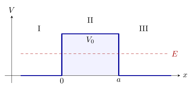
Using the same notation as for the step,
the solutions in the three regions are written
This time both exponentials must be retained in the barrier: since the region has finite length, the growing exponential presents no normalisation problem there. Continuity of and at and gives four equations,
which determine the four unknowns , , and .
6.2. The transmission coefficient
It is strictly positive for every barrier of finite width.
Proof.
Its value and derivative at then follow, using the evenness of and the oddness of :
The matching conditions at read and . Adding them eliminates the reflected amplitude:
hence
Since the potential is zero on both sides, the incident and transmitted waves have the same wavenumber, and . Using , the squared modulus of the denominator is
Finally, and , so the ratio is .
One point deserves clarification. We saw that a single real exponential carries zero current, and transmission beyond a step was zero. How, then, can the barrier transmit a non-zero current? The answer is that, inside the barrier, the wavefunction is a combination of the two exponentials, with complex coefficients. A direct calculation gives, for ,
which is non-zero whenever and do not have the same phase. The matching conditions impose precisely the combination that carries the transmitted current: there is no contradiction with the step, where the growing exponential was excluded.
6.3. Thick barrier and orders of magnitude
When the barrier is thick compared with the penetration length, , we may approximate , and the term becomes negligible in (6). This leaves
The prefactor is of order unity: everything is controlled by the exponential. This can be understood simply: the amplitude of the evanescent wave is reduced by a factor in crossing the barrier, and the probability by a factor .
This exponential dependence makes tunnelling extraordinarily sensitive to the width of the barrier and the mass of the particle. Consider an electron and a barrier exceeding its energy by eV. We find nm. For a barrier of nm, ; for a barrier of nm, it falls to about : doubling the width reduces the transmission by several tens of thousands. For a proton, is multiplied by , and the transmission through the nm barrier becomes of order , entirely negligible. Tunnelling is therefore a phenomenon of light particles and atomic distances. It underlies the scanning tunnelling microscope, whose current varies by an order of magnitude for a tip displacement of about one ångström, and it also explains radioactivity, in which an particle crosses the Coulomb barrier of the nucleus.
One point of interpretation bears emphasis. It is sometimes said that the particle temporarily “borrows” energy to cross the barrier. This picture is misleading: the Hamiltonian is time-independent, the state is stationary, and the energy is on both sides of the barrier. Tunnelling is a direct consequence of the wave nature of the wavefunction and the continuity imposed by the matching conditions.
6.4. Above the barrier
For , the barrier region is classically allowed, with wavenumber . The solution there is , and the preceding calculation remains valid if is replaced by . Since and , we obtain
The transmission is not equal to one, as it would be classically, but oscillates with energy. It becomes perfect, , when with , that is, when the width of the barrier contains an integer number of half-wavelengths: the waves reflected from the two edges of the barrier then interfere destructively. This is the same interference mechanism as in an anti-reflection coating, and a further illustration of the rules for adding amplitudes seen in Theme 1. At the threshold , the solution inside the barrier is affine; taking the limit in either formula, with , gives
6.5. An application: flash memory
Tunnelling is not merely a laboratory curiosity: it lies at the heart of the flash memory in our USB drives, phones and solid-state drives. A flash-memory cell contains a region capable of storing electric charge, separated from the rest of the transistor by an insulating layer a few nanometres thick, which acts as a potential barrier for electrons. To write or erase, a control voltage is applied that deforms the barrier and makes it sufficiently probable for electrons to cross by tunnelling. Once the voltage is removed, the barrier returns to its original shape, transmission becomes negligible again, and the charge remains trapped for years, even without a power supply. The stored charge changes the voltage required to make the transistor conduct, allowing the information to be read.
Our square barrier explains the principle: a modest change in the barrier changes the transmission by several orders of magnitude, making both rapid writing and very long retention possible. In the real device, the electric field makes the barrier triangular rather than rectangular, and charge may be stored in an isolated gate or in traps in the material; formula (6) therefore does not directly give the current through a cell. But the quantum mechanism that allows electrons to cross the insulator is indeed the one we have just calculated2.
7. Extension to three dimensions
7.1. Separation of variables
In three dimensions, the stationary equation becomes a partial differential equation:
It is generally much more difficult to solve than in one dimension. There is, however, one case that reduces directly to the preceding results: when the potential is a sum of three terms, each depending on only one coordinate, , and the boundary conditions are themselves separable. We then seek solutions in the form of a product
Substitution and division by wherever this product does not vanish gives
The first term depends only on , the second only on and the third only on . Since their sum is constant for all values of , and , each of them must be constant; denote these constants by , and , with . This gives three one-dimensional stationary equations, which we know how to solve. To assert that these products provide a basis for all states, each of the three families of solutions must also be complete, as will be the case in the example below.
7.2. The rectangular box
Consider a particle confined in the box , , , with zero potential inside and infinite walls (Figure 9). The wavefunction must vanish on all six faces. Each of the three functions , , must therefore vanish at both ends of its interval, and the results for the infinite well apply in each direction.
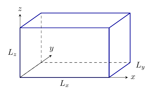
with energies
Proof.
For a cube of side , set . The ground level has energy , and is unique. The first excited level has energy , and is attained by the three states , and : it is threefold degenerate. This degeneracy is a direct consequence of the symmetry of the cube, which makes the three directions equivalent; it disappears if the box is elongated in one direction. Thus, the non-degeneracy proved on the real line does not generalise to higher dimensions.
7.3. Quantum dots and other geometries
Nanotechnology makes it possible to produce genuine “boxes” for electrons: quantum dots. These are devices ranging from a few nanometres to a few tens of nanometres in size, in which the motion of electrons is confined in all three directions. Confinement may be produced by interfaces between two semiconductor materials, by electrodes that create an electrostatic potential, or simply by the small size of a nanocrystal. As in our model, the electrons occupy discrete levels whose spacing increases as the size decreases; this makes it possible to tune the colour of the light emitted by nanocrystals by varying their size.
The rectangular-box model already explains the appearance of these levels and their dependence. For a quantitative comparison with a real dot, one would have to specify the exact shape of the confining potential, which need not be a cube with infinite walls, replace the mass of the electron by its effective mass in the material, and take interactions between electrons into account. Two neighbouring dots, coupled by tunnelling, also realise the two-site model; in Lesson 11 we shall see how to prepare a charge in one dot and observe its transfer to the other.
For a domain of arbitrary shape, the problem remains a Dirichlet problem,
but its eigenvalues depend on the geometry. A sphere or cylinder still permits separation of variables in suitable coordinates; a more general shape usually requires a numerical calculation. Likewise, a central potential, which depends only on the distance from a point, requires separation in spherical coordinates: the hydrogen atom will provide an example in Lesson 8. Before that, however, the harmonic oscillator will show us that a spectrum can also be calculated by purely algebraic means, without solving a differential equation level by level.
8. References
- [1]KIOXIAhttps://www.kioxia.com/en-jp/rd/technology/nand-flash.htmlPrésentation de la technologie des mémoires NAND Flash.