The previous lesson constructed the state space of a particle and its observables: the wave function $\psi(x)$, position acting by multiplication, momentum acting by differentiation, and the differential Hamiltonian $-\frac{\hbar^2}{2m}\frac{d^2}{dx^2}+V(x)$. We can now evolve this state. The dynamical postulate of lesson 1 applies as it stands; we need only write it in the position-space representation, which gives the Schrödinger equation in its most commonly encountered form, that of a partial differential equation.

We shall first derive a local conservation law for probability, which introduces a probability current essential for interpreting the scattering problems in the next lesson. We shall then write the stationary equation, which gives states of definite energy. We shall then study the free-particle case in full and see that a wave packet spreads over time. Finally, we shall return to Ehrenfest's theorem to understand the extent to which the centre of a packet follows Newton's laws.

Throughout this lesson, the particle has mass $m$ and the potential $V$ is real and time-independent. We shall assume that the wave functions and the potential are sufficiently regular for the derivatives written below to be meaningful.

1. The Schrödinger equation in position space

Let us start from the abstract equation of lesson 1, $i\hbar\frac{d}{dt}\ket{\psi(t)}=\hat H\ket{\psi(t)}$, and project it onto the bra $\bra x$. On the left, the time derivative commutes with the projection and gives $i\hbar\,\partial_t\psi(x,t)$, where $\psi(x,t)=\braket{x}{\psi(t)}$. On the right, $\bra x\hat H\ket{\psi(t)}$ is the function $\hat H\psi$ evaluated at $x$, which we calculated in lesson 4. We thus obtain:

Let us stress one point: this is not a new law of physics added to the postulates. It is the dynamical postulate itself, written in the position-space representation of the model constructed in lessons 3 and 4. Historically, however, it was in this form that Schrödinger proposed it in 1926, by analogy with wave optics, before the abstract formulation was established.

Note that the equation is first order in time: specifying the wave function at the initial instant is enough to determine its entire evolution, consistently with the first postulate, according to which the ket contains all the information about the state. This is an important difference from Newton's equation, which is second order and requires both the initial position and the initial velocity. The factor $i$ is also essential: it is what makes the evolution unitary, whereas a heat-diffusion equation, which has the same structure without the $i$, would cause the norm to decrease.

2. Local conservation of probability

2.1. Probability density and current

We have known since lesson 1 that unitary evolution preserves the norm of the state, that is, the total probability $\int|\psi|^2dx=1$. But it tells us more: probability cannot disappear from one region and reappear instantaneously in another distant region; it must flow continuously from one point to another, like electric charge or the mass of a fluid. This local conservation takes the form of a continuity equation.

Proof.

Differentiate the density $\rho=\psi^*\psi$ with respect to time: $$\frac{\partial\rho}{\partial t}=\psi^*\frac{\partial\psi}{\partial t}+\psi\,\frac{\partial\psi^*}{\partial t}.$$

The Schrödinger equation gives $\partial_t\psi=\frac{i\hbar}{2m}\partial_x^2\psi-\frac{i}{\hbar}V\psi$. Taking its complex conjugate, and since $V$ is real, gives $\partial_t\psi^*=-\frac{i\hbar}{2m}\partial_x^2\psi^*+\frac{i}{\hbar}V\psi^*$. Substitution yields

$$\frac{\partial\rho}{\partial t} =\frac{i\hbar}{2m}\Bigl(\psi^*\partial_x^2\psi-\psi\,\partial_x^2\psi^*\Bigr) -\frac{i}{\hbar}V\psi^*\psi+\frac{i}{\hbar}V\psi\psi^* .$$

The two potential terms cancel exactly: this is where the assumption of a real potential is used. The remaining term is an exact derivative, since

$$\frac{\partial}{\partial x}\Bigl(\psi^*\partial_x\psi-\psi\,\partial_x\psi^*\Bigr) =\partial_x\psi^*\,\partial_x\psi+\psi^*\partial_x^2\psi-\partial_x\psi\,\partial_x\psi^*-\psi\,\partial_x^2\psi^* =\psi^*\partial_x^2\psi-\psi\,\partial_x^2\psi^* .$$

Finally, $\psi^*\partial_x\psi-\psi\partial_x\psi^*=2i\operatorname{Im}(\psi^*\partial_x\psi)$, so that

$$\frac{\partial\rho}{\partial t}=\frac{i\hbar}{2m}\,\frac{\partial}{\partial x}\Bigl(2i\operatorname{Im}(\psi^*\partial_x\psi)\Bigr) =-\frac{\partial}{\partial x}\Bigl(\frac{\hbar}{m}\operatorname{Im}(\psi^*\partial_x\psi)\Bigr)=-\frac{\partial j}{\partial x}.$$

□

2.2. Balance over an interval

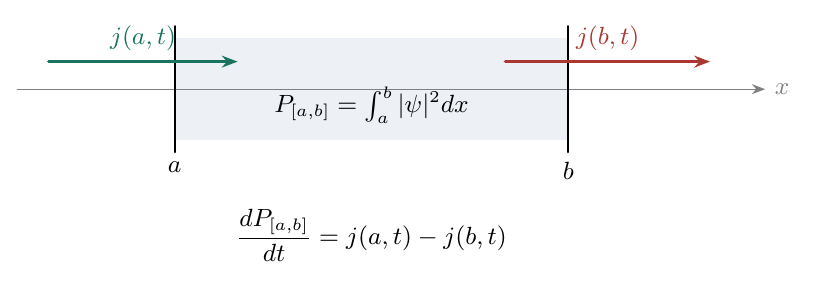
To understand the meaning of this equation, let us integrate it over an interval $[a,b]$. The term in $\partial_xj$ can be integrated directly, giving

The probability of finding the particle in the interval therefore varies only because of what crosses its boundaries: $j(a,t)$ is the probability flux entering on the left, and $j(b,t)$ that leaving on the right (see Figure 1). A positive current describes flow towards increasing $x$, and a negative current describes flow to the left. Over the whole line, the currents vanish at infinity for a normalisable state, and conservation of total probability is recovered.

2.3. The current of a plane wave

One example will be very useful in the next lesson. Consider a plane wave $\psi(x)=A\,e^{ikx}$, with $k$ real. Then $\psi^*\partial_x\psi=ik|A|^2$, and

The current is the product of the density $|A|^2$ and the classical velocity $v=p/m$ associated with the momentum $p=\hbar k$, like the flow rate of a fluid of density $\rho$ moving at velocity $v$. A wave $e^{-ikx}$ carries the opposite current. By contrast, a real wave function, or one that is real up to a constant phase, carries zero current, since $\psi^*\partial_x\psi$ is then real. This is the case, for example, of a real exponential $e^{-\kappa x}$: we shall see that this observation plays an important role in the interpretation of tunnelling.

These results show that density and flux must not be confused: two waves with the same amplitude but different velocities do not carry the same amount of probability per unit time. This must be kept in mind when defining reflection and transmission coefficients.

3. Stationary states

3.1. Separation of variables

How do we solve equation (1)? Since the potential is time-independent, a standard method for partial differential equations is first to seek particular solutions as a product

$$\psi(x,t)=\chi(t)\,\phi(x).$$

Substituting into the equation, then dividing by $\chi(t)\phi(x)$ wherever this product is non-zero, gives

$$i\hbar\,\frac{\chi'(t)}{\chi(t)} =\frac{1}{\phi(x)}\Bigl(-\frac{\hbar^2}{2m}\phi"(x)+V(x)\phi(x)\Bigr).$$

The left-hand side depends only on $t$, and the right-hand side only on $x$. For the equality to hold for all values of $t$ and $x$, both sides must equal the same constant, which we denote by $E$. This gives two decoupled equations. The time equation, $i\hbar\chi'=E\chi$, integrates immediately to $\chi(t)=e^{-iEt/\hbar}$, with the multiplicative constant absorbed into $\phi$. The spatial equation is the eigenvalue equation for the Hamiltonian, called the time-independent Schrödinger equation:

Conversely, if $\phi$ satisfies this equation, direct substitution verifies that $\psi(x,t)=e^{-iEt/\hbar}\phi(x)$ is a solution of the Schrödinger equation, including at points where $\phi$ vanishes.

We thus recover by another route the result of lesson 1: an eigenstate of the Hamiltonian evolves by acquiring only a global phase. The separation constant $E$ is the energy of this state, and is real since $\hat H$ is self-adjoint. The probability density $|\psi(x,t)|^2=|\phi(x)|^2$ is time-independent, hence the name stationary state. Note, however, that stationary does not mean motionless: the density does not change, but a constant current may flow through it, as for the plane wave (5). The continuity equation requires only $\partial_xj=0$, and hence a uniform current.

Stationary states are only particular solutions. A general solution is obtained by superposition, by decomposing the initial state over the eigenstates of the Hamiltonian. For a discrete spectrum, with $\phi_n$ of energies $E_n$,

$$\psi(x,0)=\sum_nc_n\phi_n(x) \qquad\Longrightarrow\qquad \psi(x,t)=\sum_nc_n\,e^{-iE_nt/\hbar}\,\phi_n(x),$$

with additional integrals if the spectrum includes a continuous part. Such a superposition is generally not of the form $\chi(t)\phi(x)$, and its density depends on time. Solving the dynamics therefore amounts to diagonalising the Hamiltonian: this is why the following lessons are devoted to calculating spectra.

3.2. Classically allowed and forbidden regions

Before studying examples, it is useful to know what the solutions of the time-independent equation look like. Write it in the form

$$\phi"(x)=\frac{2m}{\hbar^2}\bigl(V(x)-E\bigr)\phi(x).$$

In a region where the potential is constant, $V=V_0$, this is an equation with constant coefficients, and there are three cases.

• If $E>V_0$, set $k=\sqrt{2m(E-V_0)}/\hbar$ and the equation becomes $\phi"=-k^2\phi$. The solutions are oscillatory: $\phi(x)=Ae^{ikx}+Be^{-ikx}$, or equivalently combinations of $\cos kx$ and $\sin kx$. Classically, $E-V_0$ is the kinetic energy of the particle, and $\hbar k=\sqrt{2m(E-V_0)}$ is its momentum: we recover the de Broglie relation. This region is said to be classically allowed.
• If $E<V_0$, set $\kappa=\sqrt{2m(V_0-E)}/\hbar$ and the equation becomes $\phi"=\kappa^2\phi$. The solutions are exponential: $\phi(x)=Ce^{\kappa x}+De^{-\kappa x}$. A classical particle could not be found in this region, where its kinetic energy would be negative: it is said to be classically forbidden. Yet the wave function is generally not zero there.
• If $E=V_0$, the solutions are affine: $\phi(x)=Ax+B$.

For a slowly varying potential, this behaviour remains qualitatively true locally: the wave function oscillates where $E>V(x)$, with a local wavelength $2\pi\hbar/\sqrt{2m(E-V(x))}$ that becomes shorter as the kinetic energy increases, and behaves exponentially where $E<V(x)$. The boundary conditions and normalisability will then select, from among all these solutions, those that are physically admissible. We shall see in the next lesson that this selection is the origin of energy quantisation.

4. The free particle

4.1. Evolution in momentum space

The simplest case is that of the free particle, $V=0$. The Hamiltonian $\hat H=\hat P^2/(2m)$ then depends only on momentum. In the momentum-space representation of lesson 4, $\hat P$ acts by multiplication by $p$, so $\hat H$ acts by multiplication by $p^2/(2m)$: the Hamiltonian is diagonal in this representation. The kets $\ket p$ are generalised eigenstates of energy $p^2/(2m)$, and each component $\widetilde\psi(p,t)$ evolves independently of the others by acquiring its own phase:

This may also be obtained by writing the Schrödinger equation in the momentum-space representation, $i\hbar\,\partial_t\widetilde\psi=\frac{p^2}{2m}\widetilde\psi$, which is now merely an ordinary differential equation for each value of $p$. The momentum probability density $|\widetilde\psi(p,t)|^2$ is therefore constant: in the absence of force, the momentum distribution does not change, the quantum analogue of conservation of momentum for a free particle.

The spectrum of the free Hamiltonian is continuous: it is the set $[0,+\infty[$ of values of $p^2/(2m)$. The generalised eigenstates, the plane waves $e^{ipx/\hbar}$, are not normalisable and do not represent physical states. A physical state is a superposition of plane waves, a wave packet, whose position-space wave function is obtained by taking the inverse Fourier transform of (7).

In position space, the situation is more interesting. The different momentum components accumulate different phases $p^2t/(2m\hbar)$, and their superposition changes shape over time. Let us calculate this explicitly for an example.

4.2. Spreading of a Gaussian wave packet

Consider again the Gaussian wave packet of lesson 4, centred at $x_0$ with mean momentum $p_0$ and width $\sigma_0$,

$$\psi(x,0)=\frac{1}{(2\pi\sigma_0^2)^{1/4}} \exp\left[-\frac{(x-x_0)^2}{4\sigma_0^2}+\frac{ip_0(x-x_0)}{\hbar}\right],$$

whose Fourier transform we calculated:

$$\widetilde\psi(p,0)=\frac{1}{(2\pi\sigma_P^2)^{1/4}} \exp\left[-\frac{(p-p_0)^2}{4\sigma_P^2}\right]e^{-ipx_0/\hbar}, \qquad \sigma_P=\frac{\hbar}{2\sigma_0}.$$

According to (7), the wave function at time $t$ is

$$\psi(x,t)=\frac{1}{\sqrt{2\pi\hbar}\,(2\pi\sigma_P^2)^{1/4}}\int_\R \exp\left[-\frac{(p-p_0)^2}{4\sigma_P^2}-\frac{ip^2t}{2m\hbar}+\frac{ip(x-x_0)}{\hbar}\right]dp .$$

To obtain a Gaussian integral, set $q=p-p_0$ and expand $p^2=q^2+2p_0q+p_0^2$. The exponent becomes a quadratic polynomial in $q$:

$$-\Bigl(\frac{1}{4\sigma_P^2}+\frac{it}{2m\hbar}\Bigr)q^2 +\frac{i}{\hbar}\Bigl(x-x_0-\frac{p_0t}{m}\Bigr)q +\underbrace{\frac{ip_0(x-x_0)}{\hbar}-\frac{ip_0^2t}{2m\hbar}}_{\text{independent of }q}.$$

Introduce the characteristic time and the position of the classical centre,

$$t_d=\frac{2m\sigma_0^2}{\hbar},\qquad x_c(t)=x_0+\frac{p_0t}{m}.$$

Since $\sigma_P=\hbar/(2\sigma_0)$, the coefficient of $q^2$ can be written as $\alpha=\frac{1}{4\sigma_P^2}\bigl(1+it/t_d\bigr)$, and that of $q$ is $\beta=i(x-x_c)/\hbar$. The Gaussian integral from lesson 4, $\int_\R e^{-\alpha q^2+\beta q}\,dq=\sqrt{\pi/\alpha}\;e^{\beta^2/(4\alpha)}$, valid for $\operatorname{Re}\alpha>0$, then produces the factor

$$e^{\beta^2/(4\alpha)}=\exp\left[-\frac{(x-x_c)^2}{\hbar^2}\cdot\frac{\sigma_P^2}{1+it/t_d}\right] =\exp\left[-\frac{(x-x_c)^2}{4\sigma_0^2\,(1+it/t_d)}\right].$$

To obtain the position probability density, we need only the modulus of this factor, as the other terms are either phases or independent of $x$. Using $\operatorname{Re}\frac{1}{1+i\tau}=\frac{1}{1+\tau^2}$, we obtain

$$|\psi(x,t)|^2\propto\exp\left[-\frac{(x-x_c(t))^2}{2\sigma_0^2\bigl(1+t^2/t_d^2\bigr)}\right].$$

There is no need to calculate the constant of proportionality: since the evolution is unitary, the density remains normalised to one, which fixes it. We thus obtain the following result, illustrated in Figure 2.

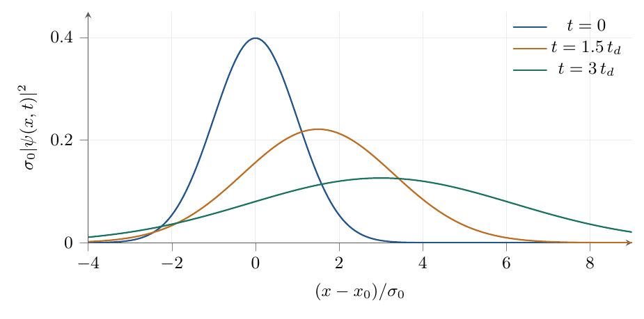
The centre of the packet therefore moves at the constant velocity $p_0/m$, like a free classical particle. But the packet spreads: its width remains approximately equal to $\sigma_0$ while $t\ll t_d$, then grows linearly with time. Indeed, for $t\gg t_d$,

$$\sigma_X(t)\simeq\frac{\sigma_0\,t}{t_d}=\frac{\hbar}{2m\sigma_0}\,t=\frac{\sigma_P}{m}\,t .$$

This last form has a simple interpretation. The packet contains momenta spread around $p_0$ with standard deviation $\sigma_P$, and hence velocities spread with standard deviation $\sigma_P/m$. A cloud of free classical particles, all starting from the same point with this spread of velocities, would spread in the same way. What is specifically quantum is that the spread of velocities is not an imperfection in the preparation that could be reduced at will: it is imposed by the initial localisation, through $\sigma_P=\hbar/(2\sigma_0)$. The narrower the packet initially, the faster it spreads. Note also that, as the packet spreads, the product $\sigma_X(t)\sigma_P$ increases: the Gaussian wave packet is a minimum-uncertainty state only at $t=0$.

A few orders of magnitude show why this spreading is never observed on our scale. For an electron initially localised to $\sigma_0=1\,\text{\AA}$, the size of an atom, we find $t_d\approx2\times10^{-16}$ s: the spreading is almost instantaneous. For a $1$ mg grain of dust localised to $1~\mu$m, we find $t_d\approx2\times10^{16}$ s, or several hundred million years.

Finally, let us stress one point: this spreading occurs under unitary Schrödinger evolution, without any measurement. It is not a loss of information: the momentum distribution is constant, and the evolution could in principle be reversed. It is the relative phases between different momentum components that rearrange themselves and deform the position probability density.

5. Ehrenfest's theorem and correspondence with Newton

5.1. Ehrenfest's equations for a particle

In lesson 3, we required the expectation values of position and momentum to obey equations analogous to Hamilton's equations, and from this we deduced the canonical relation. Let us now check that the model constructed does indeed satisfy these equations. By Ehrenfest's theorem from lesson 1, and since $\hat X$ and $\hat P$ have no explicit time dependence,

$$\frac{d\langle\hat X\rangle}{dt}=\frac{i}{\hbar}\langle[\hat H,\hat X]\rangle, \qquad \frac{d\langle\hat P\rangle}{dt}=\frac{i}{\hbar}\langle[\hat H,\hat P]\rangle .$$

We therefore need two commutators. For the first, only the kinetic energy contributes, since $V(\hat X)$ commutes with $\hat X$. Using the rule $[AB,C]=A[B,C]+[A,C]B$ and $[\hat P,\hat X]=-i\hbar\mathbf{1}$,

$$[\hat H,\hat X]=\frac{1}{2m}[\hat P^2,\hat X] =\frac1{2m}\Bigl(\hat P[\hat P,\hat X]+[\hat P,\hat X]\hat P\Bigr) =-\frac{i\hbar}{m}\hat P .$$

For the second, by contrast, the kinetic energy commutes with $\hat P$, leaving $[\hat H,\hat P]=[V(\hat X),\hat P]$. The simplest approach is to calculate it in the position-space representation, by applying the operator to a function $\psi$:

$$\bigl([V(\hat X),\hat P]\psi\bigr)(x) =V(x)\bigl(-i\hbar\psi'(x)\bigr)+i\hbar\bigl(V(x)\psi(x)\bigr)' =-i\hbar V\psi'+i\hbar V'\psi+i\hbar V\psi' =i\hbar V'(x)\psi(x).$$

As with the canonical commutator, differentiating the product produces the result. Thus $[\hat H,\hat P]=i\hbar V'(\hat X)$, and Ehrenfest's theorem gives:

The first equation says that the velocity of the centre of the packet is the mean momentum divided by the mass. The second is the analogue of Newton's second law: the change in mean momentum equals the mean force $\langle F\rangle=-\langle V'(\hat X)\rangle$. Combining the two,

$$m\,\frac{d^2\langle\hat X\rangle}{dt^2}=-\langle V'(\hat X)\rangle .$$

5.2. When does the centre of the packet follow Newton's laws?

These equations closely resemble Newton's, but with an essential difference: the right-hand side is the mean force, $\langle V'(\hat X)\rangle=\int V'(x)|\psi(x,t)|^2dx$, not the force evaluated at the mean position, $V'(\langle\hat X\rangle)$. These two quantities are not equal in general. The centre of the packet therefore does not follow an exactly classical trajectory: the force it experiences depends on how probability is distributed around it.

To estimate the discrepancy, write $\bar x=\langle\hat X\rangle$ and expand $V'$ about this point:

$$V'(x)=V'(\bar x)+V"(\bar x)(x-\bar x)+\frac12V"'(\bar x)(x-\bar x)^2+\cdots$$

Take the expectation value in the state $\psi$. The first-order term vanishes, since $\langle\hat X-\bar x\rangle=0$ by definition of $\bar x$, and the second-order term introduces the variance $\sigma_X^2=\langle(\hat X-\bar x)^2\rangle$. We obtain

$$\langle V'(\hat X)\rangle \simeq V'(\bar x)+\frac12V"'(\bar x)\,\sigma_X^2,$$

provided the following terms are negligible. Two conclusions follow.

• If the potential is at most quadratic, that is, constant, linear (constant force) or harmonic, then $V"'=0$ and all the following terms vanish: the equality $\langle V'(\hat X)\rangle=V'(\langle\hat X\rangle)$ is exact. The centre of the packet then follows the classical trajectory exactly, whatever the shape of the packet. We shall recover this result for the harmonic oscillator in lesson 7.
• For an arbitrary potential, the centre approximately follows the classical trajectory as long as the packet remains narrow compared with the scale over which the force varies, that is, as long as $|V"'|\sigma_X^2\ll|V'|$. This is one of the conditions under which classical mechanics emerges from quantum mechanics.

This second condition is not guaranteed once and for all, because we have seen that packets spread. Even in a regular potential, an initially well-localised packet eventually spreads, and quantum corrections to the trajectory of its centre eventually become significant. For a macroscopic object, the times required are astronomical, as the order of magnitude of $t_d$ showed; for an electron in an atom, by contrast, the classical description has no relevance.

5.3. What Ehrenfest does not say: the width

Ehrenfest's equations concern expectation values and by themselves say nothing about the width of the packet. For the free particle, they immediately give $\langle\hat P\rangle_t=p_0$ and $\langle\hat X\rangle_t=x_0+p_0t/m$, in agreement with the exact calculation (8), but they do not predict the spreading.

The same theorem can, however, be applied to other observables. For the free particle, take $\hat X^2$. A commutator calculation similar to the preceding one gives

$$\frac{d\langle\hat X^2\rangle}{dt}=\frac1m\langle\hat X\hat P+\hat P\hat X\rangle, \qquad \frac{d}{dt}\langle\hat X\hat P+\hat P\hat X\rangle=\frac{2}{m}\langle\hat P^2\rangle,$$

and $\langle\hat P^2\rangle$ is constant since $\hat P$ commutes with $\hat H$. The second derivative of $\langle\hat X^2\rangle$ is therefore constant, and $\langle\hat X^2\rangle$ is a quadratic polynomial in $t$. Since $\langle\hat X\rangle^2$ is also one, we obtain, for any initial state of a free particle,

$$\sigma_X^2(t)=\sigma_X^2(0)+\frac{t}{m}\Bigl(\langle\hat X\hat P+\hat P\hat X\rangle_0-2\langle\hat X\rangle_0\langle\hat P\rangle_0\Bigr)+\frac{\sigma_P^2}{m^2}\,t^2 .$$

The reader may verify these two commutation relations as an exercise. At long times, the term in $t^2$ always dominates: every free packet eventually spreads at the rate $\sigma_P/m$, as we saw in the Gaussian example, for which the linear term is zero.

The following lessons will apply these tools to particular potentials: wells and barriers, then the harmonic oscillator and the hydrogen atom. To supplement this lesson, the reader may consult D. J. Griffiths and D. F. Schroeter, Introduction to Quantum Mechanics^[1], Chapters 1 and 2, as well as the MIT notes, course 8.321, lecture 7^[2].

6. References