At the end of the previous lesson, we established the quantum model of a spinless particle moving along a line: two observables $\hat X$ and $\hat P$ satisfying the canonical commutation relation $[\hat X,\hat P]=i\hbar\mathbf{1}$, and a Hamiltonian $\hat H=\hat P^2/(2m)+V(\hat X)$. But we have not yet said anything about the objects themselves. In which Hilbert space does the state of the particle live? How do $\hat X$ and $\hat P$ act concretely on a vector in this space? These are the questions addressed in this lesson.

We shall see that the natural answer is the space $L^2(\R)$ of square-integrable functions, already encountered in theme 2, and that the wave function $\psi(x)$ introduced in lesson 1 is simply the component of the ket $\ket\psi$ on a “basis” of position states $\ket{x}$. The word basis is in quotation marks because these kets $\ket{x}$ are not genuine vectors in the Hilbert space: to manipulate them, we shall need the Dirac distribution. We shall then construct the momentum operator from translations, which will give us $\hat P=-i\hbar\, d/dx$, and then show that passing from the position-space representation to the momentum-space representation is a Fourier transform. The Hamiltonian will then take the differential form that will be the starting point for all the following lessons.

1. An infinite-dimensional space

Let us begin with a simple question: can the canonical relation be realised using matrices, as we did for spin in lesson 2? The answer is no, and the argument takes a single line. Suppose that $\hat X$ and $\hat P$ are two $n\times n$ matrices. The trace of a product does not depend on the order of its factors, $\tr(AB)=\tr(BA)$, so that

$$\tr\bigl([\hat X,\hat P]\bigr)=\tr(\hat X\hat P)-\tr(\hat P\hat X)=0, \qquad\text{whereas}\qquad \tr\bigl(i\hbar\mathbf{1}_n\bigr)=i\hbar\, n\neq0.$$

The canonical relation is therefore impossible in finite dimension: the state space of a particle is necessarily infinite-dimensional¹.

This result is consistent with what we already know. Lesson 1 taught us that a position measurement yields a continuous result $x\in\R$, with a probability density $|\psi(x)|^2$ whose integral is one. The state is therefore described by a square-integrable function, and the state space is

$$\H=L^2(\R),\qquad \braket{\phi}{\psi}=\int_\R\phi(x)^*\psi(x)\,dx .$$

Strictly speaking, two functions that are equal almost everywhere represent the same element of $L^2(\R)$, so the value of $\psi$ at an isolated point is meaningless. Throughout what follows, as physicists do, we shall work with regular functions for which these pointwise evaluations pose no problem. The “Further discussion” section at the end of the lesson explains what lies behind this convention.

2. The position-space representation

2.1. The position operator and its eigenstates

The simplest way to realise the position observable on functions is to multiply by $x$:

It is immediately clear that this operator is symmetric, since $\braket{\phi}{\hat X\psi}=\int x\,\phi^*\psi\,dx=\braket{\hat X\phi}{\psi}$, as $x$ is real. However, $x\psi(x)$ must still be square-integrable, which is not the case for every function in $L^2(\R)$: this is the domain condition $\int x^2|\psi|^2dx<\infty$ already encountered in lesson 1, which expresses the fact that the position variance is finite.

Let us now seek the eigenvectors of $\hat X$. The equation $\hat X\psi=x_0\psi$ reads

$$(x-x_0)\,\psi(x)=0\qquad\text{for every }x .$$

It requires $\psi(x)=0$ everywhere except at $x=x_0$. Such a function is zero almost everywhere and hence equal to the zero vector of $L^2(\R)$: the position operator has no eigenvector in the Hilbert space. This is the typical situation for a continuous spectrum, already discussed in theme 2. Intuitively, however, a position eigenstate should be a function “infinitely concentrated” at $x_0$, zero elsewhere, and whose integral is non-zero. No ordinary function has these properties, but they can be given a meaning as a limit.

2.2. The Dirac distribution

Consider the family of Gaussian functions

$$g_\sigma(x)=\frac{1}{\sqrt{2\pi}\,\sigma}\,e^{-x^2/(2\sigma^2)}, \qquad \int_\R g_\sigma(x)\,dx=1,$$

shown in Figure 1. As $\sigma\to0$, these functions become increasingly tall and narrow, while retaining an area equal to one. They have no limit as functions, since $g_\sigma(0)\to+\infty$. On the other hand, for any continuous bounded function $f$, the integral

$$\int_\R g_\sigma(x)\,f(x)\,dx$$

tends to $f(0)$: when $\sigma$ is very small, only the values of $f$ in the immediate vicinity of the origin contribute, and $f(x)$ may be replaced there by $f(0)$. It is this action under the integral that has a limit, and it is this limit that serves as the definition.

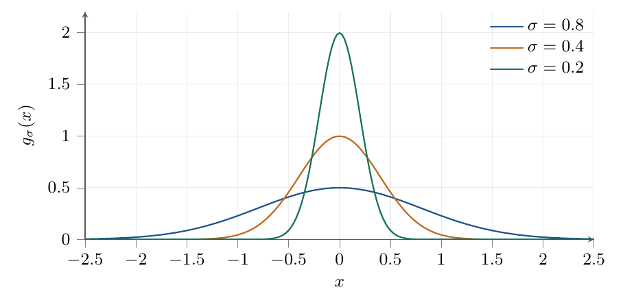
The delta is therefore not a function but a distribution, that is, an object that only has meaning when integrated against a regular function. Physicists nevertheless write it as a function and manipulate it as such under integrals; provided that definition (2) is kept in mind, this causes no difficulty. Only one thing is truly forbidden: assigning a meaning to $\delta(0)$, or to $\int\delta(x)^2dx$, neither of which exists. A few useful calculation rules are collected at the end of the lesson.

2.3. Position kets

We can now introduce, for each $x\in\R$, a ket $\ket{x}$ representing the particle “exactly at $x$”. It formally satisfies the eigenvalue equation

but does not belong to $L^2(\R)$: it is called a generalised eigenstate. Its wave function is precisely the delta, $\braket{x'}{x}=\delta(x'-x)$, as suggested by the preceding discussion.

The great advantage of these kets is that they allow us to calculate as in an orthonormal basis, replacing discrete sums by integrals and the Kronecker delta by the Dirac delta. This is the physicists' notation for the spectral families seen in theme 2:

We summarise these orthogonality and completeness relations as

The completeness relation is the basic tool in all the calculations that follow: it is inserted between a bra and a ket, and the abstract inner product becomes an integral. For example,

$$\braket{\phi}{\psi}=\bra\phi\left(\int_\R\ket{x}\bra{x}\,dx\right)\ket\psi =\int_\R\braket{\phi}{x}\braket{x}{\psi}\,dx =\int_\R\phi(x)^*\psi(x)\,dx,$$

where we used $\braket{\phi}{x}=\braket{x}{\phi}^*=\phi(x)^*$. We recover the inner product of $L^2(\R)$, which was precisely the desired result. Likewise, applying the completeness relation to the ket $\ket\psi$ itself gives its decomposition over the position kets,

the continuous analogue of $\ket\psi=\sum_nc_n\ket n$. The wave function $\psi(x)$ therefore plays the role of the components of $\ket\psi$ in the position “basis”. We say that $\psi(x)$ is the position-space representation of the ket $\ket\psi$. We shall see below that others exist.

2.4. The position operator and its projectors

The spectral decomposition of $\hat X$ is written, in this notation,

This is the continuous analogue of $\hat A=\sum_na_n\ket{a_n}\bra{a_n}$. Let us check that it does indeed reproduce the action (1). The matrix elements of $\hat X$ between position kets are

$$\bra{x}\hat X\ket{x'}=x'\braket{x}{x'}=x'\,\delta(x-x')=x\,\delta(x-x'),$$

where the last equality follows because the delta imposes $x'=x$ under the integral. Inserting the completeness relation gives

$$(\hat X\psi)(x)=\bra{x}\hat X\ket\psi =\int_\R\bra{x}\hat X\ket{x'}\braket{x'}{\psi}\,dx' =\int_\R x\,\delta(x-x')\,\psi(x')\,dx' =x\,\psi(x).$$

The circle is complete: multiplication by $x$ is indeed the operator whose generalised eigenstates are the kets $\ket{x}$.

The same formalism reproduces the measurement rules stated in lesson 1. The spectral projector associated with the interval of positions $I=[a,b]$ is

the analogue of the sum of the projectors $\ket{a_n}\bra{a_n}$ over the eigenvalues contained in $I$. Applied to a state, it gives

$$\braket{x'}{\hat\Pi_I\psi} =\int_a^b\braket{x'}{x}\braket{x}{\psi}\,dx =\int_a^b\delta(x'-x)\,\psi(x)\,dx =\mathbf 1_I(x')\,\psi(x'),$$

where $\mathbf 1_I$ is $1$ inside the interval and $0$ outside it. The projector therefore retains the part of the wave function located in $I$ and sets the rest to zero. The probability of finding the particle in $I$ and the state after measurement follow as in the discrete case:

$$P_\psi(x\in I)=\bra\psi\hat\Pi_I\ket\psi=\int_a^b|\psi(x)|^2\,dx, \qquad \ket\psi\longrightarrow\frac{\hat\Pi_I\ket\psi}{\sqrt{P_\psi(x\in I)}} .$$

These are exactly the formulae that we postulated in lesson 1. They now appear as the special case, for the position observable, of the general measurement postulates.

3. Momentum as the generator of translations

3.1. Translations

The position operator was easy to guess. Momentum is less so: how does it act on a wave function? To understand this, we shall use a property already taught to us by analytical mechanics: momentum is the quantity associated with translations in space².

Let us translate a state by a distance $a$ to the right. If the initial wave function is a packet centred at $x_0$, the translated wave function is the same packet centred at $x_0+a$. The new function therefore takes at $x$ the value that the old one took at $x-a$:

$$(T(a)\psi)(x)=\psi(x-a).$$

This operator has three important properties. It preserves the inner product, since the change of variable $u=x-a$ in the integral gives $\braket{T(a)\phi}{T(a)\psi}=\braket{\phi}{\psi}$: it is unitary. It obeys the group law $T(a)T(b)=T(a+b)$, since two successive translations compose into one. Finally, $T(0)=\mathbf{1}$ and $T(a)$ depends continuously on $a$.

We encountered exactly this situation in lesson 1 with the evolution operator $U(t)$. Stone's theorem tells us that such a continuous one-parameter unitary group can always be written as the exponential of a self-adjoint operator, called its generator. For time evolution, the generator was the Hamiltonian; for translations, we define momentum as their generator, with the convention

The factor $\hbar$ ensures that $\hat P$ has the dimensions of momentum, and the sign is chosen by analogy with $U(t)=e^{-i\hat Ht/\hbar}$.

3.2. The action of momentum

It remains to deduce the action of $\hat P$. For a small translation, we may expand both expressions for $T(a)\psi$ to first order in $a$. On the one hand, the Taylor expansion of the wave function gives

$$(T(a)\psi)(x)=\psi(x-a)=\psi(x)-a\,\psi'(x)+O(a^2).$$

On the other hand, expansion of the exponential (8) gives

$$T(a)\psi=\psi-\frac{ia}{\hbar}\hat P\psi+O(a^2).$$

Identifying the first-order terms, $-a\psi'=-ia\hat P\psi/\hbar$, we find

This, then, is the momentum operator in the position-space representation: up to a factor $-i\hbar$, it is differentiation. The factor $i$ is not an artifice; it is required for the operator to be symmetric, as we shall see. We also note that, for a wave $e^{ikx}$, the action of $\hat P$ gives $\hbar k\,e^{ikx}$: we recover the de Broglie relation $p=\hbar k$ between momentum and wave number. For another presentation of this link between translations and momentum, see the MIT notes, course 8.321, lecture 5^[1].

Proof.

Let us write the left-hand side, remembering that the inner product conjugates its first argument: the factor $-i\hbar$ becomes $+i\hbar$. Integration by parts then gives $$\begin{aligned} \braket{\hat P\phi}{\psi} &=\int_\R\bigl(-i\hbar\,\phi'(x)\bigr)^*\psi(x)\,dx =i\hbar\int_\R\phi'(x)^*\psi(x)\,dx\\ &=i\hbar\Bigl[\phi(x)^*\psi(x)\Bigr]_{-\infty}^{+\infty} -i\hbar\int_\R\phi(x)^*\psi'(x)\,dx . \end{aligned}$$

The boundary term vanishes since the functions tend to zero at infinity, leaving $\int\phi^*(-i\hbar\psi')\,dx=\braket{\phi}{\hat P\psi}$. □

Without the factor $i$, differentiation $d/dx$ alone would be antisymmetric: the same integration by parts gives $\braket{\phi'}{\psi}=-\braket{\phi}{\psi'}$. The conjugation of $i$ compensates for this sign. Note that we have established only the symmetry of $\hat P$ on regular functions; its self-adjointness requires the domain to be specified, which we shall take for granted here (see “Further discussion”). On a bounded interval, the boundary terms no longer vanish by themselves and boundary conditions will be needed: we shall see this with potential wells.

3.3. The canonical commutator

We can now check that our representation does indeed realise the canonical relation postulated in lesson 3.

Proof.

Let us calculate the two products separately. On the one hand, $$(\hat X\hat P\psi)(x)=x\,\bigl(-i\hbar\,\psi'(x)\bigr)=-i\hbar\,x\psi'(x).$$

On the other hand, $\hat P$ acts on the function $x\psi(x)$, whose derivative is calculated using the product rule:

$$(\hat P\hat X\psi)(x)=-i\hbar\,\frac{d}{dx}\bigl(x\psi(x)\bigr) =-i\hbar\,\psi(x)-i\hbar\,x\psi'(x).$$

The terms in $x\psi'$ cancel in the difference, leaving $(\hat X\hat P-\hat P\hat X)\psi=i\hbar\,\psi$. □

The calculation shows where the commutator comes from: it is the additional term produced by differentiating the factor $x$. Note that the result was not imposed by hand. We defined $\hat X$ by multiplication, and $\hat P$ as the generator of translations, and the canonical relation follows from them. The two viewpoints of lesson 3, correspondence with classical mechanics and the group structure of translations, therefore lead to the same model.

4. The momentum-space representation

4.1. Momentum eigenstates

As for position, let us seek the eigenstates of momentum. In the position-space representation, the equation $\hat P\ket p=p\ket p$ becomes a first-order differential equation for the function $\braket{x}{p}$:

$$-i\hbar\,\frac{d}{dx}\braket{x}{p}=p\,\braket{x}{p}, \qquad\text{whose solution is}\qquad \braket{x}{p}=C\,e^{ipx/\hbar}.$$

These are plane waves, with wave number $k=p/\hbar$. Their modulus $|C|$ is constant along the entire line: they are not square-integrable, and $\hat P$ likewise has no eigenvector in $L^2(\R)$. As for position, they are treated as generalised eigenstates, and the constant $C$ is chosen so as to give the same normalisation as the position kets:

$$\braket{p}{p'}=\delta(p-p').$$

To determine $C$, let us calculate this inner product by inserting the position completeness relation:

$$\braket{p}{p'}=\int_\R\braket{p}{x}\braket{x}{p'}\,dx =|C|^2\int_\R e^{i(p'-p)x/\hbar}\,dx .$$

The integral of an oscillating exponential over the whole line does not converge in the usual sense, but it has a meaning as a distribution. Regularising it by a Gaussian that tends to one, then using the Gaussian integral (18) established below, gives the identity

Indeed, the function $\sqrt{\pi/\epsilon}\,e^{-k^2/(4\epsilon)}$ is, up to a factor $2\pi$, the Gaussian $g_\sigma(k)$ of Figure 1 with $\sigma^2=2\epsilon$, and it therefore tends to $2\pi\delta(k)$. With $k=(p'-p)/\hbar$ and the rule $\delta(k)=\hbar\,\delta(p'-p)$, we find $\braket{p}{p'}=2\pi\hbar|C|^2\delta(p-p')$. We therefore choose $C=1/\sqrt{2\pi\hbar}$, real and positive:

The momentum completeness relation is established in the same way, using (11) in the opposite direction.

4.2. The Fourier transform

We now have two “bases” of the state space: the position kets and the momentum kets. The same ket $\ket\psi$ therefore has two representations: its position-space wave function $\psi(x)=\braket{x}{\psi}$, and its momentum-space wave function $\widetilde\psi(p)=\braket{p}{\psi}$. The passage from one to the other is obtained by inserting a completeness relation:

and, in the opposite direction,

We recognise the Fourier transform and its inverse, written with the variable $p=\hbar k$. We should not regard $\widetilde\psi$ as a new object: it is the same state, described by its components on another family of vectors. Here the Fourier transform is simply a change of representation, analogous to the change of basis which, in lesson 2, took us from components on $\ket{z\pm}$ to components on $\ket{x\pm}$.

Like any change of orthonormal basis, it preserves the inner product. In particular,

This is Plancherel's theorem, which can be proved by inserting (14) into the first integral and using (11). Physically, it ensures that $|\widetilde\psi(p)|^2$ is a correctly normalised probability density. By the Born rule applied to the observable $\hat P$, it is the probability density of the outcomes of a momentum measurement:

$$P_\psi(p\in J)=\bra\psi\hat\Pi^{(p)}_J\ket\psi=\int_J|\widetilde\psi(p)|^2\,dp, \qquad \hat\Pi_J^{(p)}=\int_J\ket p\bra p\,dp .$$

The Fourier integrals converge absolutely only if $\psi$ decreases sufficiently rapidly. Plancherel's theorem, which we shall assume, allows the transform to be extended to all of $L^2(\R)$ by continuity. In practice, we shall only need to calculate transforms of regular functions.

4.3. Observables in the momentum-space representation

In the momentum-space representation, the roles of $\hat X$ and $\hat P$ are interchanged: momentum now acts by multiplication, and position by differentiation.

Proof.

For the first relation, we take the transform of $\hat P\psi=-i\hbar\psi'$ and integrate by parts; the boundary term vanishes: $$\widetilde{\hat P\psi}(p)=\frac{-i\hbar}{\sqrt{2\pi\hbar}}\int_\R e^{-ipx/\hbar}\psi'(x)\,dx =\frac{i\hbar}{\sqrt{2\pi\hbar}}\int_\R\frac{d}{dx}\bigl(e^{-ipx/\hbar}\bigr)\psi(x)\,dx =p\,\widetilde\psi(p),$$

since differentiation of the exponential brings out the factor $-ip/\hbar$. For the second, we differentiate (13) with respect to $p$ under the integral:

$$i\hbar\frac{d\widetilde\psi}{dp}(p) =\frac{i\hbar}{\sqrt{2\pi\hbar}}\int_\R\left(-\frac{ix}{\hbar}\right)e^{-ipx/\hbar}\psi(x)\,dx =\frac1{\sqrt{2\pi\hbar}}\int_\R e^{-ipx/\hbar}\,x\psi(x)\,dx ,$$

which is indeed the transform of $x\psi(x)$. □

The symmetry between the two representations is almost perfect: only the sign in front of the derivative changes, which is necessary for the commutator to retain the value $i\hbar$ (check this!). We may therefore choose to work in one or the other depending on the problem. We shall see in the very next lesson that the free particle is treated much more simply in the momentum-space representation.

4.4. An example: the Gaussian wave packet

Let us calculate the Fourier transform of a Gaussian packet, centred at $x_0$, with mean momentum $p_0$:

Its position probability density $|\psi(x)|^2=e^{-(x-x_0)^2/(2\sigma_0^2)}/\sqrt{2\pi\sigma_0^2}$ is a normalised Gaussian with mean $x_0$ and standard deviation $\sigma_X=\sigma_0$: the phase $e^{ip_0(x-x_0)/\hbar}$ does not contribute to it. We shall see that it is this phase that determines the mean momentum. The calculation relies on the Gaussian integral, which we shall use frequently: for complex $\alpha$ with strictly positive real part and arbitrary complex $\beta$,

where the root with positive real part is taken. This is obtained by completing the square, $-\alpha u^2+\beta u=-\alpha\bigl(u-\beta/(2\alpha)\bigr)^2+\beta^2/(4\alpha)$, then reducing the result to $\int e^{-\alpha v^2}dv=\sqrt{\pi/\alpha}$.

In (13), set $u=x-x_0$. This gives

$$\widetilde\psi(p)=\frac{e^{-ipx_0/\hbar}}{\sqrt{2\pi\hbar}\,(2\pi\sigma_0^2)^{1/4}} \int_\R\exp\left[-\frac{u^2}{4\sigma_0^2}-\frac{i(p-p_0)u}{\hbar}\right]du .$$

This is the integral (18) with $\alpha=1/(4\sigma_0^2)$ and $\beta=-i(p-p_0)/\hbar$, equal to $2\sigma_0\sqrt\pi\,\exp[-\sigma_0^2(p-p_0)^2/\hbar^2]$. Introducing

$$\sigma_P=\frac{\hbar}{2\sigma_0},$$

and simplifying the prefactor, we obtain

The transform of a Gaussian is therefore another Gaussian. The momentum probability density $|\widetilde\psi(p)|^2$ is centred at $p_0$, confirming the role of the phase $e^{ip_0x/\hbar}$, and its standard deviation is $\sigma_P=\hbar/(2\sigma_0)$. The product of the two spreads is

$$\sigma_X\,\sigma_P=\frac\hbar2 .$$

This is exactly the bound in the Heisenberg uncertainty relation proved in lesson 3: the Gaussian packet is a minimum-uncertainty state. The mechanism behind this relation can also be seen concretely. To localise the particle, a wave function narrow in $x$ is needed, and the Fourier transform necessarily associates it with a function broad in $p$: a short signal contains many frequencies. Conversely, the position $x_0$ of the packet appears in (19) only through a phase and does not change the momentum probability density.

5. The Hamiltonian in the position-space representation

It only remains to write the Hamiltonian. The potential $V(\hat X)$ is a function of the position operator; by functional calculus, it acts on the position kets as $V(\hat X)\ket{x}=V(x)\ket{x}$, and hence by simple multiplication on wave functions:

The kinetic energy involves $\hat P^2$, that is, two successive differentiations, so that $(\hat P^2\psi)(x)=-\hbar^2\psi"(x)$. The Hamiltonian chosen in lesson 3 therefore becomes the differential operator

This expression is not quite enough to define the observable: as for $\hat P$, we must specify the functions on which it acts, and possibly impose boundary conditions so that $\hat H$ is self-adjoint. We shall specify these conditions case by case, particularly for the potential wells in lesson 6.

5.1. Extension to three dimensions

Everything above generalises without difficulty to a particle in space. We take $\H=L^2(\R^3)$, the wave function $\psi(\mathbf r)=\braket{\mathbf r}{\psi}$ and the position kets $\ket{\mathbf r}$ normalised by $\braket{\mathbf r}{\mathbf r'}=\delta^3(\mathbf r-\mathbf r')=\delta(x-x')\delta(y-y')\delta(z-z')$. Each coordinate has its own position and momentum, which act as

with $j=1,2,3$ and $(x_1,x_2,x_3)=(x,y,z)$. As in one dimension, one verifies the canonical relations

For $j\neq k$, the derivative $\partial/\partial x_k$ does not see the factor $x_j$, hence the zero commutator; and the partial derivatives commute with one another. The three (position, momentum) pairs are therefore independent. Position integrals now run over $d^3\mathbf r$; for example, the projector onto a region $\Omega$ of space is $\int_\Omega\ket{\mathbf r}\bra{\mathbf r}\,d^3\mathbf r$, and the Fourier transform involves the plane waves $\braket{\mathbf r}{\mathbf p}=e^{i\mathbf p\cdot\mathbf r/\hbar}/(2\pi\hbar)^{3/2}$.

We now have all the ingredients needed to write the Schrödinger equation of a particle in the position-space representation and study its dynamics: this will be the subject of the next lesson.

6. Further discussion: domains and generalised states

We have manipulated the kets $\ket{x}$ and $\ket p$ as vectors, even though they do not belong to the Hilbert space. This section briefly indicates how mathematicians justify these calculations. It is not needed for what follows.

A common domain for calculations.

The Schwartz space $\mathcal S(\R)$ is the set of infinitely differentiable functions which, together with all their derivatives, decrease faster than any power of $1/|x|$:

$$\mathcal S(\R)=\Bigl\{f\in C^\infty(\R)\ :\ \sup_{x\in\R}|x^mf^{(n)}(x)|<\infty\text{ for all }m,n\in\N\Bigr\}.$$

Gaussian functions belong to it. It is dense in $L^2(\R)$ and stable under differentiation, multiplication by $x$ and the Fourier transform. It is therefore a natural common domain for all the calculations in this lesson: products of $\hat X$ and $\hat P$, commutators, and integrations by parts without a boundary term. The domains on which the two operators are self-adjoint are larger:

$$D(\hat X)=\{\psi\in L^2(\R)\ :\ x\psi\in L^2(\R)\},\qquad D(\hat P)=\{\psi\in L^2(\R)\ :\ \psi'\in L^2(\R)\},$$

where the derivative is taken in the sense of distributions. It can be shown that $\hat X$ and $\hat P$ defined on $\mathcal S(\R)$ admit a unique self-adjoint extension, precisely the one defined on these domains: they are said to be essentially self-adjoint on $\mathcal S(\R)$.

The Gelfand triple.

To give generalised kets a precise status, the Hilbert space is placed between two spaces:

$$\mathcal S(\R)\subset L^2(\R)\subset\mathcal S^{\times}(\R),$$

where $\mathcal S^{\times}(\R)$ is the space of continuous antilinear forms on $\mathcal S(\R)$, which contains distributions in particular. An ordinary ket $\ket\psi$ acts on a test function $f$ as $f\mapsto\braket{f}{\psi}$; the generalised ket $\ket{x_0}$ acts as $f\mapsto f(x_0)^*$, and the ket $\ket p$ as $f\mapsto\widetilde f(p)^*$. These forms are continuous for the topology of $\mathcal S(\R)$, but not for the norm of $L^2(\R)$: this is why $\bra{x_0}$ is not an ordinary bra in the sense of the Riesz theorem. The integrals of kets and bras written in this lesson are then understood through their action on test functions. See R. de la Madrid, The role of the rigged Hilbert space in Quantum Mechanics^[2].

Uniqueness of the representation.

One may wonder whether the representation constructed here is the only possible one. The Stone—von Neumann theorem answers in the affirmative, up to unitary equivalence, for a finite number of degrees of freedom, provided that the canonical relation is formulated for the unitary groups $e^{-ia\hat P/\hbar}$ and $e^{ib\hat X/\hbar}$ (Weyl relations) rather than for the operators themselves. See P. Woit, Quantum Theory, Groups and Representations^[3].

Some formulae for the delta.

The following identities are understood under an integral against a test function, and are proved by a change of variable in (2):

$$\delta(-x)=\delta(x),\qquad \delta(ax)=\frac1{|a|}\,\delta(x)\quad(a\neq0),\qquad x\,\delta(x)=0 .$$

If $f$ is regular and has only simple zeros $x_i$,

$$\delta(f(x))=\sum_i\frac{\delta(x-x_i)}{|f'(x_i)|}.$$

Finally, the derivative of the delta is defined by integration by parts:

$$\int_\R f(x)\,\delta'(x-x_0)\,dx=-f'(x_0).$$

7. References