The harmonic oscillator is undoubtedly the most important model in the whole of physics, both classical and quantum. The reason is simple: near a stable minimum, any regular potential resembles a parabola. The small oscillations of a pendulum, the vibrations of atoms about their equilibrium positions in a molecule or a crystal, and even, as we shall see much later, the modes of the electromagnetic field, are all described, to a first approximation, by a harmonic oscillator.

In this lesson, we shall calculate its spectrum and eigenstates. We could proceed as we did for the wells in the previous lesson, by solving the stationary differential equation. Instead, we shall follow an algebraic method, due to Dirac, which is both more elegant and more instructive. It is based on factorising the Hamiltonian using two operators, known as ladder operators, which allow us to move from one energy level to the next. We shall see that the positivity of certain operators, a direct consequence of the notion of adjoint, is enough to determine the spectrum completely. We shall return to the position-space representation only at the end, to write the wave functions explicitly, and shall then recover the Hermite functions already encountered in Theme 2.

1. The model

1.1. The neighbourhood of a minimum

Let us work in one dimension, and consider a regular potential $V(x)$ with a minimum at $x_0$, where $V'(x_0)=0$ and $V"(x_0)>0$. The Taylor expansion near this point is

The linear term is absent because $x_0$ is a minimum. Let us choose the origin of position at $x_0$ and the origin of energy at $V(x_0)$. If the particle remains sufficiently close to the minimum for higher-order terms to be negligible, its Hamiltonian is that of a harmonic oscillator:

The angular frequency $\omega$ is that of small classical oscillations about the minimum. In what follows, we shall treat this Hamiltonian as exact. When it is used to approximate another potential, however, one must bear in mind that the approximation becomes less accurate for highly excited states, which explore regions farther from the minimum where higher-order terms, known as anharmonic terms, are no longer negligible.

1.2. The natural scales

Before beginning any calculation, it is useful to identify the scales of the problem. They are fixed by the three constants $m$, $\omega$ and $\hbar$, from which one can form only a single energy, $\hbar\omega$, and a single length,

We can go further and estimate the ground-state energy using the uncertainty relation. In a state with standard deviations $\sigma_X$ and $\sigma_P$, and expectation values equal to zero by symmetry, the expectation value of the energy is

where we have used $\sigma_P\geq\hbar/(2\sigma_X)$. The first term, the kinetic term, penalises excessively strong localisation; the second, the potential term, penalises excessive spreading. The minimum of the right-hand side as a function of $\sigma_X$ is attained for $\sigma_X^2=\hbar/(2m\omega)=\ell^2/2$, and is exactly $\hbar\omega/2$ (check this!). No state can therefore have an expectation value of the energy below $\hbar\omega/2$. We shall see that this bound is attained: it is the exact ground-state energy. The particle cannot be at rest at the bottom of the well, for the same reason as in the infinite well of Lesson 6.

For what follows, it is convenient to measure lengths in units of $\ell$ and momenta in units of $\hbar/\ell$. Introduce the dimensionless operators

The canonical relation $[\hat X,\hat P]=i\hbar\mathbf{1}$ becomes $[\tilde X,\tilde P]=i\mathbf{1}$, and the Hamiltonian takes the highly symmetric form

2. Ladder operators

2.1. The idea of factorisation

For real numbers $x$ and $p$, we would factorise the sum of two squares using complex numbers: $x^2+p^2=(x-ip)(x+ip)$. Let us try to do the same with the operators $\tilde X$ and $\tilde P$. Since they do not commute, we must carefully preserve the order of the factors when expanding:

Thus the factorisation works up to a constant term, which arises from the commutator. Reversing the order of the factors similarly gives $(\tilde X+i\tilde P)(\tilde X-i\tilde P)=\tilde X^2+\tilde P^2+\mathbf{1}$. It is precisely this small difference between the two orders that will generate the entire structure of the spectrum.

To lighten the notation, we do not place hats on these new operators. The factor $1/\sqrt2$ is chosen to simplify the commutator below, and the names given to these operators will be justified by their properties. Note that $a^\dagger$ is indeed the adjoint of $a$: since $\tilde X$ and $\tilde P$ are self-adjoint, taking the adjoint merely conjugates the factor $i$. In contrast, $a$ is not self-adjoint, and therefore does not represent an observable. Nor is it a unitary operator: $a^\dagger$ is not the inverse of $a$.

2.2. The oscillator algebra

Thus, up to a constant, the Hamiltonian is the operator $N$. Diagonalising $\hat H$ amounts to diagonalising $N$: if $N\ket\lambda=\lambda\ket\lambda$, then $\ket\lambda$ is an eigenstate with energy $\hbar\omega(\lambda+1/2)$. The rest of the argument consists in determining the possible values of $\lambda$, using only relations (5).

3. The spectrum

3.1. Positivity of the number operator

A first piece of information follows directly from the definition of $N$ as the product of an operator and its adjoint. For any state $\ket\psi$,

The operator $N$ is therefore positive. In particular, its eigenvalues are non-negative: if $N\ket\lambda=\lambda\ket\lambda$ with $\ket\lambda$ normalised, then $\lambda=\bra\lambda N\ket\lambda\geq0$. We thus recover, exactly, the bound $\langle\hat H\rangle\geq\hbar\omega/2$ obtained above from the uncertainty relation.

3.2. Moving up and down the ladder

Now take a normalised eigenstate $\ket\lambda$ of $N$, and consider what becomes of $a\ket\lambda$ and $a^\dagger\ket\lambda$. The commutator $[N,a]=-a$ may be written $Na=aN-a$, so that

Thus, if $a\ket\lambda$ is not the zero vector, it is an eigenstate of $N$ with eigenvalue $\lambda-1$. Similarly, $Na^\dagger=a^\dagger N+a^\dagger$ gives

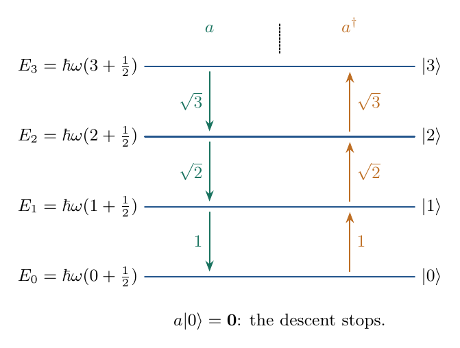
The operator $a$ therefore moves one step down the ladder of eigenvalues, that is, it lowers the energy by one quantum $\hbar\omega$, while $a^\dagger$ moves it up one step. This is the origin of the name ladder operators, and of their names as annihilation and creation operators for a quantum of energy.

It is also important to know the norm of the resulting vectors. Once again, it is calculated using the adjoint:

where we have used $aa^\dagger=a^\dagger a+\mathbf{1}$. These two formulae have an important consequence: the lowered state $a\ket\lambda$ is zero if and only if $\lambda=0$, whereas the raised state $a^\dagger\ket\lambda$ is never zero. One can therefore never be stopped while moving up the ladder, but one can be stopped while moving down it, and only at the level $\lambda=0$.

3.3. An integer spectrum

We can now determine the possible eigenvalues. The idea is simple: starting from an eigenvalue $\lambda$ and moving down the ladder gives the values $\lambda-1$, $\lambda-2$, and so on, which would eventually become negative, something forbidden by the positivity of $N$. The descent must therefore stop, and it can do so only on reaching exactly zero.

Note the power of this argument: we have used only the commutation relation and positivity, without ever writing a differential equation. The argument does not yet prove, however, that every integer is indeed an eigenvalue, nor that there is only one eigenstate for each eigenvalue, nor that these states form a basis. These three points require us to construct the ground state explicitly, which we shall do in the position-space representation.

4. The ground state

The bottom of the ladder is a state $\ket0$ with eigenvalue $0$. By (6), $\norm{a\ket0}^2=0$, and it is therefore characterised by

The right-hand side is the zero vector, not a physical state: the equation simply expresses the fact that there is no lower level. Conversely, any state satisfying (7) satisfies $N\ket0=a^\dagger a\ket0=0$.

To solve this equation, move to the position-space representation, where $\hat P=-i\hbar\,d/dx$. From definition (4), we have $i\ell\hat P/\hbar=\ell\,d/dx$, and the ladder operators become first-order differential operators:

The ground-state equation is therefore the first-order differential equation

This is the entire advantage of the factorisation: instead of solving the stationary Schrödinger equation, which is second order, it is enough to solve a first-order equation, which can be integrated immediately.

The ground state is therefore a Gaussian of width $\ell$. Its probability density $|\phi_0|^2\propto e^{-x^2/\ell^2}$ has standard deviation $\sigma_X=\ell/\sqrt2$, which is the value that minimised the energy in our estimate based on the uncertainty relation. It is a Gaussian packet of the type studied in Lesson 4, with $x_0=p_0=0$ and $\sigma_0=\ell/\sqrt2$, and is therefore a minimum-uncertainty state.

For an electron, an atom or a molecule, $\ell$ is typically of the order of a fraction of an ångström to a few ångströms. For a laboratory pendulum, by contrast, $\ell$ is absurdly small: with $m=1$ kg and $\omega=1$ rad s$^{-1}$, one finds $\ell\approx10^{-17}$ m, and the zero-point energy $\hbar\omega/2$ is entirely unobservable.

5. Excited states

5.1. Recursive construction

Starting from the normalised ground state $\ket0$, let us move up the ladder. The vector $a^\dagger\ket0$ is an eigenstate of $N$ with eigenvalue $1$, and its norm is $\sqrt{0+1}=1$ by (6). We may therefore set $\ket1=a^\dagger\ket0$. The next vector, $a^\dagger\ket1$, has eigenvalue $2$, but its norm is $\sqrt2$: to obtain a normalised state, we must divide by this factor, and

Similarly, $\ket3=\frac{1}{\sqrt3}a^\dagger\ket2=\frac{1}{\sqrt{3!}}(a^\dagger)^3\ket0$, and so on. The factorial that appears is not a convention: it compensates for the norms accumulated at each upward step.

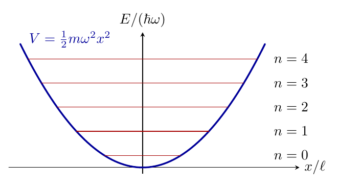
The spectrum of the oscillator has a remarkable structure: the levels are equally spaced, separated by $E_{n+1}-E_n=\hbar\omega$ (Figure 2). This is very different from the infinite well, where the gaps increased as $2n+1$: the more slowly the potential widens, the closer together the levels become at high energy. The integer $n$ counts the number of quanta $\hbar\omega$ above the ground state; hence the name number operator for $N$. Note, however, that here these quanta are not particles. The model still describes a single particle in a potential, and $n$ simply indexes its energy levels. It is in quantum field theory that these quanta acquire the status of particles, for example photons for the modes of the electromagnetic field.

5.2. The wave functions

The excited states are obtained by repeatedly applying the differential operator $a^\dagger$ to the Gaussian (9). In the dimensionless variable $\xi=x/\ell$, we have $a^\dagger=(\xi-d/d\xi)/\sqrt2$ and $d\phi_0/d\xi=-\xi\phi_0$. Thus

Repeating the operation, with $\frac{d}{d\xi}(\xi\phi_0)=(1-\xi^2)\phi_0$, gives

At each step, the same Gaussian is multiplied by a polynomial whose degree increases by one. The general formula involves the Hermite polynomials $H_n$, defined by the recurrence relation

which gives, for example, $H_2(\xi)=4\xi^2-2$. It can be shown that

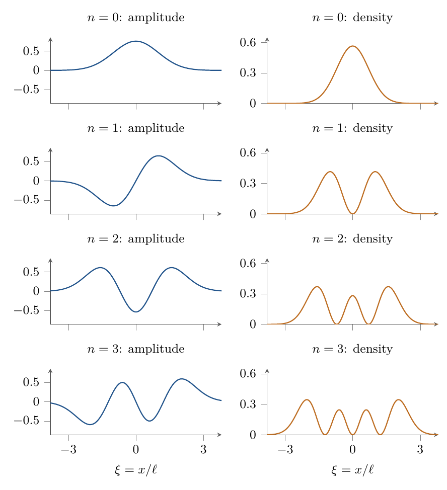
as is readily verified for $n=1$ and $n=2$ using the preceding expressions. These are the Hermite functions that we presented in Theme 2 as an example of a Hilbert basis of $L^2(\R)$, noting that they were the eigenstates of the harmonic oscillator (Figure 3). The figure shows that $\phi_n$ has $n$ nodes, like the states of the infinite well, and that it is even for even $n$ and odd for odd $n$, as it must be for an even potential with non-degenerate levels (cf. Lesson 6).

Note also that the wave functions extend beyond the classically allowed region $|x|\leq x_n$, where $x_n=\ell\sqrt{2n+1}$ is the amplitude of a classical oscillation with energy $E_n$: as in the finite well, the wave function penetrates the forbidden region, where it decays as a Gaussian.

6. Expectation values and fluctuations

The algebraic method also makes it very easy to calculate expectation values, without ever calculating an integral. It is enough to invert definitions (4) to express position and momentum in terms of the ladder operators:

By (11), these two operators connect a state $\ket n$ only to its immediate neighbours $\ket{n-1}$ and $\ket{n+1}$. This is a selection rule that we shall encounter again: only the matrix elements $\bra{n\pm1}\hat X\ket n$ are non-zero.

It follows that the energy is divided equally between its kinetic and potential contributions in each eigenstate:

as for the time average of a classical oscillation. As $n$ increases, the position distribution broadens, and the momentum spread also increases: only the ground state minimises the product of the two, without either spread vanishing.

7. Dynamics

What happens for a state that is not an eigenstate? Since the potential is quadratic, we saw in Lesson 5 that Ehrenfest's theorem gives exactly classical equations for the expectation values:

The centre of any wave packet therefore oscillates exactly like a classical particle, at angular frequency $\omega$: $\langle\hat X\rangle(t)=\langle\hat X\rangle_0\cos\omega t+\frac{\langle\hat P\rangle_0}{m\omega}\sin\omega t$.

This can be checked for the example of the superposition $\ket{\psi(0)}=(\ket0+\ket1)/\sqrt2$. By Lesson 1, it evolves as

Using (14) and $\bra0\hat X\ket1=\ell/\sqrt2$, we find

which indeed oscillates at the classical angular frequency. More generally, all the energy differences $E_n-E_m=(n-m)\hbar\omega$ are integer multiples of $\hbar\omega$. All the relative phases therefore return to their initial value after the classical period $2\pi/\omega$, and every state of the oscillator is periodic, up to a global phase. This property, specific to the equally spaced spectrum, makes the harmonic oscillator the quantum system closest to its classical analogue. One can even construct Gaussian packets that oscillate without changing shape, the coherent states, which we shall study later.

8. Scope of the model

The vibration of a diatomic molecule near its equilibrium separation provides a direct application. The relevant coordinate is then the distance between the two nuclei, and the mass is the reduced mass of the pair. The harmonic approximation predicts equally spaced vibrational levels, separated by $\hbar\omega$, which are observed in infrared spectroscopy. For the HCl molecule, for example, $\hbar\omega\approx0.36$ eV. The actual levels become slightly closer together as $n$ increases, because of the anharmonic terms in the potential, which eventually allow the molecule to dissociate; the departure from the harmonic law provides a precise measure of these terms. The vibrations of the atoms in a crystal about their equilibrium positions can likewise be decomposed into a large number of independent oscillators, whose quanta are called phonons.

The model also applies to a particle trapped near the minimum of a trap, such as an ion in an electromagnetic trap or an atom in an optical trap, and more generally to any system whose Hamiltonian reduces, over the energy range under study, to the sum of a quadratic kinetic energy and a quadratic potential. In three dimensions, an isotropic harmonic potential $\frac12m\omega^2(x^2+y^2+z^2)$ separates into three independent oscillators, like the box in Lesson 6, and its levels $\hbar\omega(n_x+n_y+n_z+3/2)$ are degenerate.

Finally, let us retain the role played by the adjoint throughout this lesson. It gave us the positivity of $N$, from which quantisation follows; it fixed the norms of the lowered and raised states, and hence the factors $\sqrt n$ and $\sqrt{n+1}$; and it is the Hilbert-space structure that allowed us to construct an orthonormal basis of eigenstates. We shall encounter the same algebraic method again, with a ladder bounded on both sides this time, for angular momentum and spin in Lesson 10.

9. References